Astronomic and geodetic positioning

Before satellites, every geodetic position on Earth was ultimately tied to the stars. Latitudes came from the altitudes of stars on the meridian, longitudes from comparing local star time with the time at Greenwich, and azimuths from the position of Polaris. Triangulation carried these positions across continents, and the resulting networks became the national datums. GNSS has replaced astronomy for positioning, but the astronomic observations measure something GNSS cannot: the direction of the actual plumb line. That direction is what every leveled instrument is aligned with, and comparing it with the ellipsoid normal reveals the shape of the geoid. This lesson explains astronomic coordinates, how they are observed, how classical datums were built from them, and the Laplace equation that connects astronomic and geodetic azimuths.

To show the difference, a university geodesy group lent Coulee Geomatics a digital zenith camera for one clear October night. Mounted on pillar CR1, it photographed stars near the zenith, while Theo Martel also observed a north and a south star on the meridian with a precise theodolite and timed the observations against GNSS time. The results differ from the NAD83(2011) coordinates of the pillar by a few arcseconds. That difference is not an error.

Astronomic coordinates

The astronomic latitude \(\Phi\) of a point is the angle between the plumb line (the direction of gravity) and the plane of the celestial equator, which is parallel to the Earth's equatorial plane. The astronomic longitude \(\Lambda\) is the angle between the astronomic meridian plane of the point, which contains the plumb line and a parallel to the rotation axis, and the reference meridian plane. The astronomic azimuth \(A\) of a line is measured clockwise from astronomic north in the plane perpendicular to the plumb line, the plane in which a leveled theodolite turns. These quantities are defined by gravity and the Earth's rotation, not by any ellipsoid. They can be observed anywhere, without any datum.

Geodetic coordinates \(\varphi\), \(\lambda\) and geodetic azimuth \(\alpha\) are defined by the ellipsoid normal instead. Because the plumb line and the normal differ by the deflection of the vertical, typically a few arcseconds and up to a minute in mountains, astronomic and geodetic values differ by the same amount. Lesson 10 treats the deflection itself; here the task is to observe the astronomic quantities.

The celestial sphere and latitude

Astronomers describe star positions on the celestial sphere, an imaginary sphere of very large radius centered on the observer. The celestial poles lie on the extension of the Earth's rotation axis, and the celestial equator is the projection of the Earth's equator. A star's declination \(\delta\) is its angular distance north or south of the celestial equator, and its right ascension is measured eastward along the celestial equator, usually in hours. Star catalogs, now based on space astrometry, give these coordinates to a few milliarcseconds.

At a point with astronomic latitude \(\Phi\), the celestial pole stands at an altitude \(\Phi\) above the horizon, and the zenith, the upward direction of the plumb line, has declination \(\Phi\). A star crossing the meridian south of the zenith at zenith distance \(z\) therefore satisfies \(\Phi = \delta + z\), and one crossing north of the zenith satisfies \(\Phi = \delta - z\). Measuring zenith distances of stars on the meridian is the oldest precise method of finding latitude.

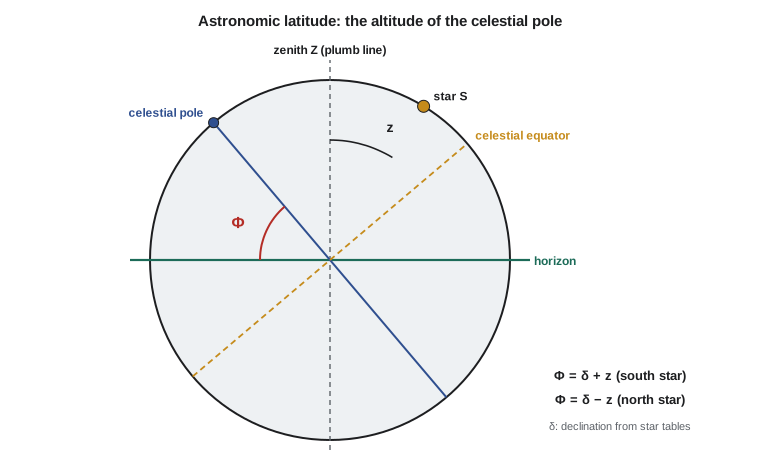
The main error source is atmospheric refraction, which bends starlight so that stars appear higher than they are by about \(58''\tan z\) at moderate zenith distances. The refraction depends on temperature and pressure and is uncertain by a few percent. The Sterneck or Talcott method pairs a star south of the zenith with one north of it at nearly equal zenith distance: the refraction corrections enter the two latitude formulas with opposite signs, so most of their uncertainty cancels in the mean. Zenith cameras go further, observing only stars within a degree or so of the zenith, where refraction is negligible, and achieve accuracies of about 0.1″.

Longitude is time

The Earth turns through 15° of longitude per hour of sidereal time. A star crosses the local meridian when the local sidereal time equals its right ascension, so timing a transit gives the local sidereal time at that instant. If the Greenwich sidereal time at the same instant is known, the astronomic longitude follows:

where LAST and GAST are the local and Greenwich apparent sidereal times, converted from hours to degrees. Determining longitude was historically the hard part, because it required carrying Greenwich time to the observer. Chronometers, telegraph signals and radio time signals each improved it in turn. Today the time comes from GNSS, and the conversion from atomic time to Earth rotation time is the subject of lesson 11. One second of time in longitude is 15″, so a timing error of a millisecond corresponds to 0.015″, about 0.3 m on the ground at the site.

Astronomic azimuth

Azimuth is found by observing the horizontal angle between a reference mark and a star whose azimuth at the instant of observation can be computed from its right ascension, declination, the observer's latitude and the sidereal time. Polaris is the classic choice in the northern hemisphere, because it moves slowly in azimuth and its azimuth is insensitive to timing errors. Observations of the Sun are less precise but were widely used for property surveys. The azimuth obtained is astronomic, referred to the plumb line. Gyrotheodolites, which find north from the Earth's rotation, also measure astronomic azimuth, and they are still used to orient tunnels and mine surveys where no GNSS signal reaches.

Classical geodetic datums

A classical horizontal datum was built by triangulation from an initial point. At that point, astronomic latitude, longitude and azimuth were observed and, together with chosen values for the deflection of the vertical (often zero) and the geoid height, defined how the reference ellipsoid was placed relative to the Earth. Triangulation then carried positions outward through chains of triangles, scaled by measured base lines.

The North American Datum of 1927 used the Clarke 1866 ellipsoid with its initial point at Meades Ranch, Kansas, and covered the United States, Canada and Mexico. Because the ellipsoid was placed to fit the geoid near Kansas, its center was offset from the Earth's center of mass by more than 200 m. NAD83, adopted in the United States and Canada in 1986, abandoned the initial point. It placed the GRS80 ellipsoid at the Earth's center of mass as determined from satellite Doppler observations and VLBI, and it combined the old triangulation with modern measurements in one adjustment. Positions in Montana moved by several tens of meters between NAD27 and NAD83.

Triangulation networks controlled direction poorly: small errors in each triangle swung the azimuth of the chain. To stop the swing, astronomic azimuths were observed at Laplace stations spaced through the network and converted to geodetic azimuths by the Laplace equation.

The Laplace equation

A theodolite leveled at a station measures horizontal angles in the plane perpendicular to the plumb line and refers azimuths to astronomic north. The geodetic azimuth, referred to the ellipsoid normal and the geodetic meridian, differs because the two verticals are tilted relative to each other. To first order, the relation is

where \(\xi = \Phi - \varphi\) and \(\eta = (\Lambda - \lambda)\cos\varphi\) are the deflection components and \(z\) is the zenith distance of the target. The first correction accounts for the different meridians, and it requires an astronomic longitude: this is why Laplace stations needed both longitude and azimuth observations. The second correction depends on the deflection and the inclination of the line of sight, and vanishes for horizontal sightings. For lines inclined by a few degrees and deflections of a few arcseconds, it reaches tenths of a second.

# Astronomic latitude, longitude and azimuth at pillar CR1, compared with geodetic values
import math

def dms(d, m, s): return math.copysign(abs(d) + m / 60 + s / 3600, d)
def sec(x): return x * 3600
def show(x):
    sgn = "-" if x < 0 else ""; x = abs(x)
    d = int(x); m = int((x - d) * 60); s = (x - d - m / 60) * 3600
    return sgn + str(d) + " " + str(m).zfill(2) + " " + format(s, "05.2f")

def refraction(z):                  # mean refraction in arcsec for zenith distance z (deg), standard air
    return 58.3 * math.tan(math.radians(z)) - 0.067 * math.tan(math.radians(z)) ** 3

# 1. Latitude from a north and a south star crossing the meridian (Sterneck pair)
dec_S, z_S = dms(18, 21, 4.62), dms(29, 8, 46.83)     # star south of the zenith
dec_N, z_N = dms(80, 47, 33.94), dms(33, 16, 31.72)      # star north of the zenith
zS = z_S + refraction(z_S) / 3600                     # observed z is too small: add refraction
zN = z_N + refraction(z_N) / 3600
Phi = ((dec_S + zS) + (dec_N - zN)) / 2
print("latitude from south star", show(dec_S + zS), " from north star", show(dec_N - zN))
print("astronomic latitude PHI =", show(Phi), " (refraction south minus north:", round(refraction(z_S) - refraction(z_N), 2), "arcsec)")

# 2. Longitude: local apparent sidereal time minus Greenwich apparent sidereal time at the same instant
LAST = dms(4, 24, 48.13) * 15       # star's right ascension when it crossed the local meridian, in degrees
GAST = dms(11, 49, 59.940) * 15     # Greenwich sidereal time at that instant, from the time signal
Lam = (LAST - GAST + 180) % 360 - 180
print("astronomic longitude LAMBDA =", show(Lam))

# 3. Compare with the geodetic coordinates of CR1 (GNSS, NAD83(2011))
phi, lam = dms(47, 30, 21.6152), -dms(111, 17, 52.0473)
xi = sec(Phi - phi)
eta = sec(Lam - lam) * math.cos(math.radians(phi))
print("deflection components: xi =", round(xi, 2), "arcsec, eta =", round(eta, 2), "arcsec")

# 4. Laplace equation: astronomic azimuth of CR1 -> CR2 reduced to a geodetic azimuth
A_astro = dms(84, 53, 2.29)                         # from the star observations and the angle to CR2
z = dms(89, 56, 48.0)                                # zenith distance to CR2
alpha = A_astro - sec(Lam - lam) * math.sin(math.radians(phi)) / 3600
alpha -= (xi * math.sin(math.radians(A_astro)) - eta * math.cos(math.radians(A_astro))) / math.tan(math.radians(z)) / 3600
print("Laplace geodetic azimuth CR1 -> CR2 =", show(alpha), "(GNSS gives", show(84.8850) + ")")
print("correction applied =", round(sec(alpha - A_astro), 2), "arcsec; across 560 m that is",
      round(560.1 * math.radians((alpha - A_astro)) * 1000, 1), "mm")

latitude from south star 47 30 23.95  from north star 47 30 23.98
astronomic latitude PHI = 47 30 23.96  (refraction south minus north: -5.74 arcsec)
astronomic longitude LAMBDA = -111 17 57.15
deflection components: xi = 2.35 arcsec, eta = -3.45 arcsec
Laplace geodetic azimuth CR1 -> CR2 = 84 53 06.05 (GNSS gives 84 53 06.00)
correction applied = 3.76 arcsec; across 560 m that is 10.2 mm

The two stars give latitudes that agree to 0.03″ after refraction corrections of 32″ and 38″. Their mean, the astronomic latitude, is 47° 30′ 23.96″, which is 2.35″ north of the geodetic latitude. The transit time gives an astronomic longitude 5.10″ west of the geodetic longitude, which at this latitude is an east–west deflection component of −3.45″. The Laplace correction of almost 4″ brings the astronomic azimuth to within 0.05″ of the GNSS azimuth. In a real campaign, many stars would be observed through the night, the instrument errors would be eliminated by reversing it, and the standard deviation of the result would be a few tenths of a second.

Astronomy in modern geodesy

Astronomic positioning is no longer used to fix coordinates, but it remains important in three ways. First, astronomic observations measure the deflection of the vertical directly, and digital zenith cameras are used to validate geoid models with an independent, high-resolution data set; along a profile, deflections integrate to geoid height differences, as lesson 10 shows. Second, every leveled instrument works in the astronomic frame, so precise networks that combine terrestrial angles with GNSS must account for the difference, especially in mountains. Third, the celestial reference frame defined by distant quasars, observed by VLBI, is what links the Earth's orientation to inertial space, and it underpins GNSS orbits and the time scales of lesson 11.

For the land surveyor, the most common encounter with astronomy is in old records. Bearings in many original property and right-of-way surveys were derived from solar or Polaris observations and are astronomic, often of limited accuracy and referred to the meridian at the time and place of observation. Retracing such surveys means understanding what the original bearing meant, not simply rotating it to grid north.