
GCP-221 · Lesson 3 of 12 · 19 min
Joins, aggregations and window functions
▶ Video coming soon A video version of this lesson is on the way.
The Wednesday session on October 14 starts with a follow-up from Lena. The September list was useful, she says, but she now wants three more things: sales by product category for each region, each store's rank within its region, and a running total of sales through the month so managers can see whether they are on pace. Each request needs a different SQL tool. Category sales need a join and an aggregation; ranks and running totals need window functions.
Joins: bringing tables together
Birchline's sales table records a SKU and a store ID, but not the product category or the store's region. Those live in reference tables. A join combines rows from two tables where a condition is true, usually where key columns match. The type of join decides what happens to rows that have no match on the other side.
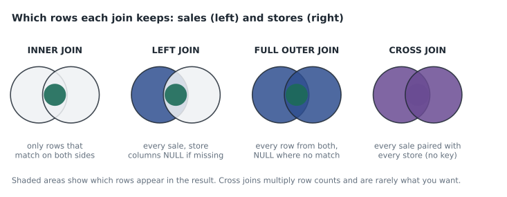
| Join | Keeps | Typical use |
|---|---|---|
| INNER JOIN | Only rows with a match on both sides | Sales with their product details, when every SKU should exist |
| LEFT JOIN | Every row of the left table; right-side columns NULL when there is no match | Keeping all sales even if a SKU is missing from the catalog |
| FULL OUTER JOIN | Every row from both tables | Reconciling two lists to find what is missing from each |
| CROSS JOIN | Every combination of rows | Building a calendar of every store for every day |
The choice between inner and left joins is a decision about what the report should do with incomplete data, and it should be made deliberately. An inner join to the product table silently drops sales of any SKU that is missing from the catalog, so totals shrink without warning. A left join keeps those sales with a NULL category, and the report can show them as "Uncategorized" with COALESCE. Ravi's rule: use a left join from the fact table to a reference table unless you are certain every key matches, and check the count of NULLs afterward.
The fan-out trap
The most dangerous join mistake does not cause an error. It makes totals too large. If the right-hand table has more than one row for a key, each left row is repeated once for every match, and any SUM over the left table's columns is multiplied. This is called fan-out.
Mateo meets it straight away. The product table he joins to has one row per SKU, but the promotions table has one row per SKU per promotion, and three tent SKUs were in two September promotions each. Joining sales to promotions doubles every sale of those tents, and the category total for camping jumps by tens of thousands of dollars. The fix is to know the grain of each table, meaning what one row represents, and to aggregate the many-rows side to the join key before joining, or to join to a version with one row per key.
import sqlite3
db = sqlite3.connect(":memory:")
db.executescript("""
CREATE TABLE sales (sku TEXT, net_sales REAL);
INSERT INTO sales VALUES ('TNT-2P', 300), ('TNT-2P', 300), ('STK-AL', 20), ('TNT-4P', 500);
CREATE TABLE promos (sku TEXT, promo TEXT);
INSERT INTO promos VALUES ('TNT-2P', 'Long Weekend'), ('TNT-2P', 'Fall Camp'), ('TNT-4P', 'Fall Camp');
""")
q = lambda s: db.execute(s).fetchall()
print("true total:", q("SELECT SUM(net_sales) FROM sales"))
print("after joining promos (fan-out):",
      q("SELECT SUM(s.net_sales) FROM sales s LEFT JOIN promos p USING (sku)"))
print("joined to one row per SKU:",
      q("""SELECT SUM(s.net_sales) FROM sales s
LEFT JOIN (SELECT sku, COUNT(*) AS n_promos FROM promos GROUP BY sku) p USING (sku)"""))true total: [(1120.0,)] after joining promos (fan-out): [(1720.0,)] joined to one row per SKU: [(1120.0,)]
What this code does
Showing how a join can inflate a total. Four sale lines worth 1,120 dollars are joined to a promotions table that lists one tent twice. The first total is the true one; the second is too large because each sale of that tent is repeated for each of its promotions; the third is correct again because the promotions were first reduced to one row per product before joining.
A quick defensive habit catches fan-out: count the rows before and after a join. If a left join to a reference table returns more rows than the fact table had, some key on the right is duplicated.
Aggregations and grouping
Aggregate functions such as SUM, COUNT, AVG, MIN and MAX reduce many rows to one value per group. Every column in the SELECT list must either be inside an aggregate or appear in GROUP BY. BigQuery also supports GROUP BY ROLLUP, which adds subtotal rows, and GROUPING SETS for several groupings in one pass. Lena's category report uses ROLLUP to give each region's categories, a total for each region, and a grand total in one result.
SELECT
  st.region,
  COALESCE(pr.category, "Uncategorized")       AS category,
  SUM(s.net_sales)                             AS net_sales,
  COUNT(DISTINCT s.sale_id)                    AS lines
FROM `bl-data-prod.curated.sales`        AS s
LEFT JOIN `bl-data-prod.reference.products` AS pr USING (sku)
JOIN `bl-data-prod.reference.stores`     AS st USING (store_id)
WHERE s.sale_date BETWEEN "2026-09-01" AND "2026-09-30"
  AND s.channel = "store"
GROUP BY ROLLUP (st.region, category)
ORDER BY st.region, category;
-- Rows with a NULL category are region subtotals; the row with NULL region is the grand total.
ROLLUP produces NULLs in the grouping columns for its subtotal rows, which can be confused with real NULLs. The GROUPING() function returns 1 for a subtotal row and 0 otherwise, so a report can label subtotals clearly.
Window functions
A window function computes a value for each row using a set of related rows, called the window, without collapsing the rows into one. That is the difference from GROUP BY. A window is described with OVER, which can contain PARTITION BY to split rows into groups, ORDER BY to order rows within each group, and a frame to say which rows around the current one to include.
| Need | Window function | Example |
|---|---|---|
| Rank within a group | RANK, DENSE_RANK, ROW_NUMBER | Rank stores by sales within each region |
| Running total | SUM(...) OVER (ORDER BY ...) | Month-to-date sales |
| Moving average | AVG(...) OVER (ORDER BY ... ROWS BETWEEN 6 PRECEDING AND CURRENT ROW) | 7-day average of daily sales |
| Previous or next value | LAG, LEAD | Change from the previous week |
| Share of a total | x / SUM(x) OVER (PARTITION BY ...) | A store's share of its region |
| Keep one row per group | ROW_NUMBER with QUALIFY | Latest price for each SKU |
The three ranking functions differ only in how they treat ties. ROW_NUMBER gives every row a different number, breaking ties arbitrarily unless the ORDER BY is complete. RANK gives tied rows the same number and then skips, so two stores tied for first are followed by third. DENSE_RANK gives tied rows the same number without skipping, so the next store is second. For a league table shown to managers, RANK is usually what people expect.
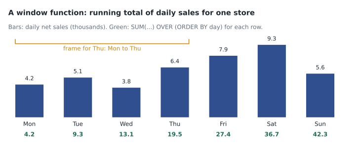
Lena's pacing view uses a running total within each store, ordered by date, and compares it with the store's monthly target. The rank within region uses RANK partitioned by region. Both are computed in one query, and QUALIFY could filter the result to, say, the top three stores in each region without another layer of nesting.
WITH daily AS (
  SELECT store_id, sale_date, SUM(net_sales) AS net_sales
  FROM `bl-data-prod.curated.sales`
  WHERE sale_date BETWEEN "2026-10-01" AND "2026-10-13" AND channel = "store"
  GROUP BY store_id, sale_date
)
SELECT
  d.store_id, st.region, d.sale_date, d.net_sales,
  SUM(d.net_sales) OVER (PARTITION BY d.store_id ORDER BY d.sale_date)          AS month_to_date,
  AVG(d.net_sales) OVER (PARTITION BY d.store_id ORDER BY d.sale_date
                         ROWS BETWEEN 6 PRECEDING AND CURRENT ROW)              AS avg_7_day,
  RANK() OVER (PARTITION BY st.region, d.sale_date ORDER BY d.net_sales DESC)   AS rank_in_region
FROM daily AS d
JOIN `bl-data-prod.reference.stores` AS st USING (store_id);
Window functions run after WHERE and GROUP BY, which is why the query aggregates to daily totals in a CTE first. A window over raw sale lines would rank individual purchases, not stores.
Checking a window by hand
New window functions should be checked against a small case worked out by hand. Mateo uses SQLite, which supports the same window syntax, to confirm the running total and the ranks on a few rows before trusting the BigQuery result on forty stores.
import sqlite3
db = sqlite3.connect(":memory:")
db.execute("CREATE TABLE d (store TEXT, day INT, sales REAL)")
rows = [("A", 1, 4.2), ("A", 2, 5.1), ("A", 3, 3.8), ("A", 4, 6.4),
        ("B", 1, 5.0), ("B", 2, 5.1), ("B", 3, 4.0), ("B", 4, 6.4)]
db.executemany("INSERT INTO d VALUES (?, ?, ?)", rows)
sql = """
SELECT store, day, sales,
       ROUND(SUM(sales) OVER (PARTITION BY store ORDER BY day), 1) AS running,
       RANK()       OVER (PARTITION BY day ORDER BY sales DESC)    AS rnk,
       DENSE_RANK() OVER (PARTITION BY day ORDER BY sales DESC)    AS dense,
       ROUND(sales - LAG(sales) OVER (PARTITION BY store ORDER BY day), 1) AS change
FROM d ORDER BY store, day
"""
for r in db.execute(sql):
print(r)('A', 1, 4.2, 4.2, 2, 2, None)
('A', 2, 5.1, 9.3, 1, 1, 0.9)
('A', 3, 3.8, 13.1, 2, 2, -1.3)
('A', 4, 6.4, 19.5, 1, 1, 2.6)
('B', 1, 5.0, 5.0, 1, 1, None)
('B', 2, 5.1, 10.1, 1, 1, 0.1)
('B', 3, 4.0, 14.1, 1, 1, -1.1)
('B', 4, 6.4, 20.5, 1, 1, 2.4)What this code does
Checking window results on a few rows by hand. Two stores have four days of sales each. For every row the output shows the running total within the store, the store's rank among the two stores that day with RANK and DENSE_RANK, and the change from the store's previous day. Day 2 and day 4 have ties, which show how the ranking functions treat equal values, and the first day of each store has no previous day, so its change is empty.
On day 4 both stores sold 6.4, so both rank first. With only two stores, RANK and DENSE_RANK give the same result; with a third store below them, RANK would give it 3 and DENSE_RANK would give it 2. The first change value for each store is NULL, because LAG has no previous row to look at. Explaining these details in a report footnote avoids questions later.
Common mistakes
MistakeJoining a fact table to a table with several rows per key and summing.
InsteadKnow each table's grain; aggregate the many-rows side to the key first, and compare row counts before and after the join.
MistakeUsing an inner join to a reference table by default.
InsteadUse a left join unless every key is certain to match, and show unmatched rows as a labeled group.
MistakeApplying a window function to raw rows when the question is about daily totals.
InsteadAggregate in a CTE first, then apply the window.
MistakeUsing ROW_NUMBER for a league table with ties.
InsteadUse RANK or DENSE_RANK so tied stores share a position.
One last check before Lena sees the category report: Mateo compares the grand total from the ROLLUP query with the total from v_store_daily for the same month. They agree to the dollar, which confirms that the left join kept every sale and that no join fanned out. This single reconciliation catches most join mistakes and takes a minute.
Worked problem
Ranks with ties
In the West region on October 13, store sales were: store 31, 9,400 dollars; store 33, 8,100; store 36, 9,400; store 38, 7,600. What do RANK and DENSE_RANK give each store, ordered by sales from highest?
Show solution
- Sort: 9,400 (stores 31 and 36), 8,100 (store 33), 7,600 (store 38).
- RANK: stores 31 and 36 share 1; the next rank skips to 3 for store 33; store 38 is 4.
- DENSE_RANK: stores 31 and 36 share 1; store 33 is 2; store 38 is 3.
- ROW_NUMBER would give 1 and 2 to stores 31 and 36 in an unpredictable order unless a tie-breaker is added.
Answer: RANK: 31 and 36 are 1, 33 is 3, 38 is 4. DENSE_RANK: 31 and 36 are 1, 33 is 2, 38 is 3.
Summary and key terms
- Joins combine tables: inner joins keep only matches, left joins keep every row of the left table, full outer joins keep everything, and cross joins pair every row with every other.
- Choose inner or left deliberately, and check unmatched rows.
- Fan-out happens when the right table has several rows per key and inflates sums; knowing each table's grain and comparing row counts prevents it.
- GROUP BY ROLLUP adds subtotals.
- Window functions compute values over related rows without collapsing them: RANK, DENSE_RANK and ROW_NUMBER rank rows, SUM OVER gives running totals, frames give moving averages, and LAG and LEAD compare with nearby rows.
- Aggregate first, then apply windows.
- Join
- Combining rows from two tables where a condition is true.
- LEFT JOIN
- A join that keeps every row of the left table.
- Fan-out
- Repeated rows caused by joining to a table with several matches per key, which inflates totals.
- Grain
- What one row of a table represents.
- ROLLUP
- A GROUP BY option that adds subtotal and grand total rows.
- Window function
- A function that computes a value for each row from a set of related rows.
- Frame
- The rows around the current row that a window function includes.
- LAG
- A window function that returns a value from an earlier row.
Practice problems
Work each problem on paper first, then reveal the answer to check.
A left join from sales to products returns more rows than the sales table has. What does that suggest?
Show answer
Some SKUs appear more than once in the products table, so rows are fanning out.
What is the difference between RANK and DENSE_RANK?
Show answer
Both give ties the same rank; RANK then skips numbers, DENSE_RANK does not.
Which window clause gives a 7-day moving average?
Show answer
ROWS BETWEEN 6 PRECEDING AND CURRENT ROW, ordered by date.
Why aggregate to daily totals before ranking stores?
Show answer
Window functions run after grouping; ranking raw lines would rank individual purchases.
Lesson quiz · 5 questions
Score 60% or more to complete this lesson.
Create a free account to save your progress, take quizzes and earn a certificate.