
GCP-221 · Lesson 2 of 12 · 20 min
Writing SQL in BigQuery
▶ Video coming soon A video version of this lesson is on the way.
Friday's session, on October 9, begins with a real request. Lena Okafor wants to know which stores had the weakest September compared with August, and she wants the answer before her Monday call with the regional managers. Ravi uses the request to walk Mateo through writing BigQuery SQL properly: readable, correct about dates and missing values, and cheap to run.
GoogleSQL and the shape of a query
BigQuery's SQL dialect is called **GoogleSQL**, and it follows the ANSI standard closely. Older material mentions **legacy SQL**, with square brackets around table names; it still exists for old jobs but should not be used for new work, and the console uses GoogleSQL by default. Table names in GoogleSQL go in backticks when they contain hyphens, as Birchline's project name does: `bl-data-prod.curated.sales`.
A query is written in one order and evaluated in another. You write SELECT first, but BigQuery starts with FROM and the joins, then filters rows with WHERE, groups them, filters the groups with HAVING, computes the SELECT list, filters window results with QUALIFY, sorts and finally limits. Knowing the evaluation order explains several error messages that puzzle new analysts.
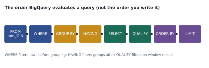
Two consequences matter every day. First, a column alias defined in SELECT cannot be used in WHERE, because WHERE is evaluated before SELECT; repeat the expression, or compute it in a common table expression first. Second, an aggregate such as SUM cannot appear in WHERE, because rows are filtered before they are grouped; a condition on a total belongs in HAVING.
Building the September comparison
Ravi and Mateo build Lena's query in steps, each in a common table expression (CTE), introduced with WITH. A CTE gives a name to an intermediate result so the final SELECT reads like a short story rather than a nest of brackets.
-- Store sales, September vs August 2026, store channel only
WITH monthly AS (
  SELECT
    store_id,
    DATE_TRUNC(sale_date, MONTH)                 AS month,
    SUM(net_sales)                               AS net_sales
  FROM `bl-data-prod.curated.sales`
  WHERE sale_date BETWEEN "2026-08-01" AND "2026-09-30"   -- partition filter
    AND channel = "store"
    AND NOT is_refund
  GROUP BY store_id, month
),
pivoted AS (
  SELECT
    store_id,
    SUM(IF(month = "2026-08-01", net_sales, 0))  AS aug,
    SUM(IF(month = "2026-09-01", net_sales, 0))  AS sep
  FROM monthly
  GROUP BY store_id
)
SELECT
  p.store_id,
  s.store_name,
  s.region,
  p.aug,
  p.sep,
  ROUND(SAFE_DIVIDE(p.sep - p.aug, p.aug), 3)    AS change_ratio
FROM pivoted AS p
JOIN `bl-data-prod.reference.stores` AS s USING (store_id)
ORDER BY change_ratio
LIMIT 10;
Each part of the query earns its place. The WHERE clause filters on sale_date, the column the table is partitioned by, so BigQuery reads only August and September instead of almost four years. DATE_TRUNC turns every date into the first day of its month, which makes grouping by month simple. The second CTE pivots the two months into columns with conditional aggregation, SUM(IF(...)), a pattern worth memorizing. And SAFE_DIVIDE returns NULL instead of an error if a store had no August sales, which would otherwise stop the whole query on a division by zero.
Before sending anything, Ravi asks the question every analyst should ask of a ranking: is the comparison fair? September has 30 days and August has 31, and in 2026 August has five Saturdays while September has four. A store that did exactly as well on every day would still show a small drop. They add a version that compares average daily sales instead of totals, and two of the ten weakest stores drop off the list. The note to Lena explains both views.
Dates and times
Dates cause more wrong answers than any other part of SQL. GoogleSQL has four related types, and choosing the right one matters.
| Type | Holds | Example | Use for |
|---|---|---|---|
| DATE | A calendar day | 2026-09-30 | Business days, partition columns, monthly reports |
| DATETIME | A day and clock time with no time zone | 2026-09-30 21:15:00 | Local times as printed on a receipt |
| TIMESTAMP | An exact moment, stored in UTC | 2026-10-01 01:15:00 UTC | Events that must be compared across time zones |
| TIME | A clock time with no date | 21:15:00 | Opening hours |
The most common trap is converting a TIMESTAMP to a DATE without saying which time zone. DATE(sale_ts) uses UTC, so a sale at 21:15 in Columbus on September 30 becomes October 1. Birchline's curated.sales table stores both sale_ts and a sale_date already converted to the store's local day, and analysts are told to filter and group on sale_date. When converting yourself, write DATE(sale_ts, "America/New_York").
Other useful functions include DATE_ADD and DATE_SUB to move dates, DATE_DIFF to count days between two dates, EXTRACT(DAYOFWEEK FROM sale_date) to find the weekday, where 1 is Sunday and 7 is Saturday, and FORMAT_DATE to print a date for a report. Filtering on a range with BETWEEN includes both ends, so BETWEEN "2026-09-01" AND "2026-09-30" covers all of September for a DATE column. For a TIMESTAMP column, the safe pattern is a half-open range: sale_ts >= start AND sale_ts < next_start, which does not miss the last second of the day.
NULL: the value that is not a value
NULL means a value is missing or unknown, and it does not behave like zero or an empty string. Any comparison with NULL is neither true nor false but NULL, so WHERE discount = NULL finds nothing; the correct test is WHERE discount IS NULL. Aggregates ignore NULLs: AVG(discount) is the average of the rows that have a discount, not of all rows. COUNT(*) counts rows, while COUNT(discount) counts rows where discount is not NULL. COALESCE returns the first value that is not NULL and is the usual way to supply a default.
Ravi demonstrates these rules with a tiny table in SQLite, which runs in the browser and behaves the same way as BigQuery for NULLs and grouping. The data is five sale lines from two stores.
import sqlite3
db = sqlite3.connect(":memory:")
db.execute("CREATE TABLE sales (store_id INT, net_sales REAL, discount REAL)")
db.executemany("INSERT INTO sales VALUES (?, ?, ?)", [
    (12, 80.0, None), (12, 120.0, 10.0), (12, 40.0, None),
    (15, 300.0, 30.0), (15, 60.0, 0.0),
])
q = lambda sql: db.execute(sql).fetchall()

print("rows with discount = NULL:", q("SELECT COUNT(*) FROM sales WHERE discount = NULL"))
print("rows with discount IS NULL:", q("SELECT COUNT(*) FROM sales WHERE discount IS NULL"))
print("COUNT(*) vs COUNT(discount):", q("SELECT COUNT(*), COUNT(discount) FROM sales"))
print("AVG(discount) vs AVG(COALESCE(discount, 0)):",
      q("SELECT AVG(discount), AVG(COALESCE(discount, 0)) FROM sales"))
print("stores with total over 250 (HAVING):",
q("SELECT store_id, SUM(net_sales) FROM sales GROUP BY store_id HAVING SUM(net_sales) > 250"))rows with discount = NULL: [(0,)] rows with discount IS NULL: [(2,)] COUNT(*) vs COUNT(discount): [(5, 3)] AVG(discount) vs AVG(COALESCE(discount, 0)): [(13.333333333333334, 8.0)] stores with total over 250 (HAVING): [(15, 360.0)]
What this code does
Showing how missing values and grouping behave, using a small in-memory database. It loads five sale lines, two of which have no discount recorded. The results show that testing "equals NULL" finds nothing, that counting a column skips missing values, that the average discount changes depending on whether missing means zero, and that a condition on a store's total must be written with HAVING.
The average discount line is the one that matters for reports. Without COALESCE the average is about 13.33, the mean of the three recorded discounts. With missing values treated as zero it is 8.0. Which is right depends on what a missing discount means in the source. At Birchline, the till leaves the field empty when no discount applies, so zero is correct, and the curated table already stores 0. The lesson is to know what NULL means in each column before averaging it.
Writing SQL that others can read
Most queries are read many more times than they are written. Birchline's SQL style guide asks for a few simple habits: keywords in capitals, one column per line in long SELECT lists, a comment on any filter that is not obvious, meaningful aliases rather than single letters for anything longer than a few lines, and CTEs instead of deep nesting. Queries saved for others start with a comment that says what the query answers and who asked.
BigQuery also supports query parameters, written as @name, which let a saved query or an application supply values such as a date range without editing the SQL. Parameters make queries safer, because values are never pasted into the text, and they make saved queries reusable.
-- Weekly store sales for any week: supply @week_start when running
SELECT store_id, SUM(net_sales) AS net_sales
FROM `bl-data-prod.curated.sales`
WHERE sale_date BETWEEN @week_start AND DATE_ADD(@week_start, INTERVAL 6 DAY)
GROUP BY store_id;

-- bq query --use_legacy_sql=false --parameter=week_start:DATE:2026-09-28 ...
Useful functions for analysts
A handful of functions cover most everyday analysis. It is worth knowing them by name, because exam scenarios often describe a need and offer functions as answers.
| Need | Function | Example |
|---|---|---|
| Avoid division by zero | SAFE_DIVIDE(a, b) | SAFE_DIVIDE(returns, sales) |
| Default for missing values | COALESCE(x, default) | COALESCE(discount, 0) |
| Conditional value | IF(cond, a, b) or CASE WHEN | IF(units < 0, "refund", "sale") |
| Count distinct values (exact) | COUNT(DISTINCT x) | COUNT(DISTINCT session_id) |
| Count distinct values (fast estimate) | APPROX_COUNT_DISTINCT(x) | Visitors on a 3-billion-row table |
| Text matching | LIKE, REGEXP_CONTAINS | REGEXP_CONTAINS(page, r"/tents/") |
| Rounding money | ROUND(x, 2) | ROUND(net_sales, 2) |
| Percentiles | APPROX_QUANTILES(x, 100)[OFFSET(50)] | Median basket size |
The approximate functions deserve a comment. APPROX_COUNT_DISTINCT and APPROX_QUANTILES use clever summaries instead of keeping every value, so they run much faster on very large tables, with an error that is usually well under one in 100. For a dashboard of daily web visitors, the estimate is fine. For a figure that will be reconciled with finance, use the exact function.
Common mistakes
MistakeWriting WHERE total > 1000 after grouping.
InsteadConditions on aggregates go in HAVING; WHERE filters rows before grouping.
MistakeTesting for missing values with = NULL.
InsteadUse IS NULL or IS NOT NULL.
MistakeConverting a TIMESTAMP to a DATE without a time zone.
InsteadGive the zone, such as DATE(ts, "America/New_York"), or use a column already in local dates.
MistakeComparing monthly totals for months of different lengths.
InsteadCompare average daily figures, or the same days of the week, when the months differ.
Reading and fixing error messages
Most SQL errors in BigQuery fall into a few families, and reading the message carefully usually points straight at the fix. "Unrecognized name: change_ratio" in a WHERE clause means an alias was used before it exists, the evaluation-order problem described earlier. "SELECT list expression references column region which is neither grouped nor aggregated" means a column in the SELECT list must be added to GROUP BY or wrapped in an aggregate such as ANY_VALUE. "No matching signature for operator = for argument types: DATE, STRING" means a value of the wrong type is being compared; a literal such as "2026-09-30" is usually converted automatically, but a string column is not, and needs CAST or PARSE_DATE. "Division by zero" is solved with SAFE_DIVIDE, and "Not found: Table" usually means a missing project name or a dataset in a different location.
The editor helps before you run anything. The validator underlines errors as you type, and the message appears in the same place as the bytes estimate. Ravi's advice is to fix the first error first: later errors are often consequences of the first one, and disappear once it is fixed. He also suggests building long queries one CTE at a time, running each step with a small date range, and checking its row count before adding the next. A query built and tested in pieces is much easier to debug than one written in a single pass and run for the first time against four years of data.
Finally, results deserve the same scrutiny as errors. A query that runs without complaint can still be wrong, and the quickest checks are simple: does the total for one store and one day match what the store reported? Does the number of rows make sense, forty stores times thirty days for a monthly daily table? Are there NULLs where you did not expect them? Mateo now ends every new query by comparing one figure with a source he trusts before sending anything to Lena.
Worked problem
Fair comparison of two months
Store 22 sold 186,000 dollars in August 2026 (31 days) and 183,000 dollars in September 2026 (30 days). Did its daily performance fall?
Show solution
- August average per day: 186,000 / 31 = 6,000 dollars.
- September average per day: 183,000 / 30 = 6,100 dollars.
- Change in the daily average: (6,100 - 6,000) / 6,000 = 0.0167, about 1.7 in 100.
- The monthly total fell by 3,000 dollars only because September is a day shorter.
Answer: No. The store's average daily sales rose slightly, by about 1.7 in 100, even though the monthly total fell.
Summary and key terms
- GoogleSQL is BigQuery's standard SQL dialect; legacy SQL should not be used for new work.
- Queries are evaluated in the order FROM, WHERE, GROUP BY, HAVING, SELECT, QUALIFY, ORDER BY, LIMIT, so aliases cannot be used in WHERE and aggregates belong in HAVING.
- CTEs make long queries readable.
- DATE, DATETIME, TIMESTAMP and TIME hold different things, and converting a timestamp to a date needs a time zone.
- NULL is not zero: test it with IS NULL, and remember that aggregates skip it.
- SAFE_DIVIDE, COALESCE and conditional aggregation are everyday tools, and query parameters make saved queries reusable and safe.
- GoogleSQL
- BigQuery's ANSI-compliant SQL dialect.
- Common table expression
- A named intermediate result defined with WITH.
- HAVING
- A clause that filters groups after aggregation.
- SAFE_DIVIDE
- Division that returns NULL instead of failing when the divisor is zero.
- COALESCE
- A function that returns its first argument that is not NULL.
- TIMESTAMP
- An exact moment in time, stored in UTC.
- Conditional aggregation
- Aggregating only rows that meet a condition, such as SUM(IF(...)).
- Query parameter
- A named value such as @week_start supplied when a query runs.
Practice problems
Work each problem on paper first, then reveal the answer to check.
Why can a SELECT alias not be used in WHERE?
Show answer
Because WHERE is evaluated before SELECT, so the alias does not exist yet.
A sale at 21:15 local time on September 30 in Eastern time shows up on October 1. Why?
Show answer
The TIMESTAMP was converted to a DATE in UTC instead of the local time zone.
What does COUNT(discount) count?
Show answer
The rows where discount is not NULL.
When is APPROX_COUNT_DISTINCT a good choice?
Show answer
For very large tables where a small estimation error is acceptable, such as dashboard visitor counts.
Lesson quiz · 5 questions
Score 60% or more to complete this lesson.
Create a free account to save your progress, take quizzes and earn a certificate.