
ENGG-160 · Lesson 9 of 12 · 28 min
Testing, measurement and experiments
Lesson 2 introduced verification and validation, and Lesson 7 the prototypes that make testing possible. This lesson looks at testing itself: how to plan a test that answers a real question, how measurements go wrong, how to describe the spread in repeated measurements and attach an honest uncertainty to a result, how uncertainties in measured inputs carry through to a calculated answer, and how designed experiments find the effects of several factors at once far more efficiently than changing one thing at a time. It closes with acceptance testing and the integrity of test records. These skills apply equally to a student design project, a laboratory course, a product qualification program and the commissioning of a building or plant.
Planning a test
A test is an experiment designed to answer a question, and a good test plan makes that question explicit before any equipment is set up. A useful plan states:
- The objective: the question to be answered or the requirement to be verified, traced to the specification (Lesson 2).
- The pass and fail criteria: what result would count as success, decided before the test so the result cannot be rationalized afterwards.
- The test article: which prototype or production unit, in what configuration and condition.
- The variables: what will be changed (independent variables), what will be measured (dependent variables), and what will be held constant (controlled variables).
- The method: the setup, loads or inputs, sequence, number of repetitions, instruments and their calibration.
- Safety: hazards of the test itself, such as stored energy in springs, pressure vessels, high voltage and parts that may fracture, and the controls for them.
- Data recording and analysis: what will be recorded, how, and how results will be analyzed.
Writing the plan forces the team to think about what could go wrong and whether the test can actually answer the question. Many failed tests were well executed but poorly designed: the loads did not represent service conditions, the measurement could not resolve the effect of interest, or nothing was held constant.
Measurement: accuracy, precision and resolution
Every measurement differs from the true value by some error. Three properties of a measurement system describe how well it performs:
- Resolution: the smallest change the instrument can display, such as 0.01 mm on a digital caliper.
- Precision (repeatability): how closely repeated measurements of the same quantity agree.
- Accuracy: how close measurements are to the true value.
An instrument can be precise but inaccurate (readings tightly grouped around the wrong value) or accurate on average but imprecise (readings scattered around the right value). Resolution is not accuracy: a scale that displays four decimal places may still be wrong in the first.
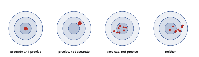
Errors fall into two kinds. Random errors vary unpredictably from one reading to the next, from electrical noise, small variations in setup and the limits of reading a scale; they can be reduced by averaging repeated measurements. Systematic errors push every reading the same way: an uncalibrated instrument, a zero offset, a thermocouple not in good contact, a load cell read at the wrong temperature, or a consistent mistake in method. Averaging does not reduce systematic errors; calibration against a known standard, careful method and independent checks do. Calibration records, traceable through a chain of comparisons to national measurement standards, are required for test results that will be used for certification or safety.
Describing repeated measurements
When a measurement is repeated n times, its central value is described by the mean and its spread by the standard deviation s. The mean of n measurements is more reliable than any single one: its standard error is \(s/\sqrt{n}\). A 95 % confidence interval for the true mean, assuming the measurements are roughly normal and free of systematic error, is:
where t is taken from Student's t distribution for n − 1 degrees of freedom; for large n it approaches 1.96, but for small samples it is larger (2.262 for ten measurements, 4.303 for three). Averaging four measurements halves the standard error; averaging a hundred cuts it by ten.
import math, statistics as st

# 1. Repeated measurements: tip deflection of a prototype bracket under 500 N (mm)
d = [1.82, 1.79, 1.85, 1.81, 1.88, 1.80, 1.83, 1.86, 1.78, 1.84]
n, mean, s = len(d), st.mean(d), st.stdev(d)
se = s / math.sqrt(n)
t95 = 2.262                                   # Student t, 9 degrees of freedom, 95 percent
print(f"Deflection: mean {mean:.3f} mm, SD {s:.3f} mm, 95% CI {mean:.3f} +/- {t95 * se:.3f} mm")

# 2. Propagating uncertainty: density of a block from mass and three dimensions
m, um = 118.4, 0.1                            # g
L, W, H, ul = 50.12, 30.05, 10.02, 0.02       # mm, caliper uncertainty each
rho = m / (L * W * H) * 1000                  # g/cm3
rel = math.sqrt((um / m) ** 2 + (ul / L) ** 2 + (ul / W) ** 2 + (ul / H) ** 2)
print(f"Density {rho:.3f} g/cm3 +/- {rho * rel:.3f} ({rel:.2%}); thickness term alone {ul / H:.2%}")

# 3. A two-level factorial test: strength (N) of 3D-printed brackets
runs = {("20%", 2): 410, ("60%", 2): 520, ("20%", 4): 560, ("60%", 4): 640}   # (infill, walls)
infill = ((runs[("60%", 2)] + runs[("60%", 4)]) - (runs[("20%", 2)] + runs[("20%", 4)])) / 2
walls = ((runs[("20%", 4)] + runs[("60%", 4)]) - (runs[("20%", 2)] + runs[("60%", 2)])) / 2
inter = ((runs[("60%", 4)] - runs[("20%", 4)]) - (runs[("60%", 2)] - runs[("20%", 2)])) / 2
print(f"Main effect of infill {infill:+.0f} N, of wall count {walls:+.0f} N, interaction {inter:+.0f} N")Deflection: mean 1.826 mm, SD 0.032 mm, 95% CI 1.826 +/- 0.023 mm Density 7.846 g/cm3 +/- 0.018 (0.23%); thickness term alone 0.20% Main effect of infill +95 N, of wall count +135 N, interaction -15 N
The first result reports the deflection as 1.826 ± 0.023 mm at 95 % confidence: the true mean deflection very probably lies between 1.80 and 1.85 mm, assuming no systematic error. If the requirement were "deflection shall not exceed 2.0 mm", the bracket passes with a clear margin; if it were "shall not exceed 1.83 mm", ten measurements are not enough to say, and either more tests or a design change would be needed.
Propagating uncertainty
Most results are calculated from several measured quantities, each with its own uncertainty. If the uncertainties are independent and random, they combine by root-sum-square rather than simple addition, because they are unlikely all to err in the same direction at once. For a result that is a product or quotient of measured quantities, such as density \(\rho = m/(LWH)\), the relative uncertainties combine:
For a sum or difference, the absolute uncertainties combine the same way. For a quantity raised to a power, the relative uncertainty is multiplied by the power: the area of a circle from its diameter has twice the relative uncertainty of the diameter.
The second result in the code shows the practical value of this: the density of the steel block is 7.846 ± 0.018 g/cm³, and almost all the uncertainty comes from the thinnest dimension, the 10 mm thickness, where the caliper's 0.02 mm uncertainty is a larger fraction. To improve the result, measure the thickness more precisely, with a micrometer; measuring the mass more precisely would achieve nothing. Uncertainty analysis tells you where to spend effort.
Worked problem
Uncertainty in a flow measurement
Flow rate is found by timing how long a pump takes to fill a 20.0 L bucket. The volume is known to ±0.2 L and the time, 31.5 s, to ±0.5 s (reaction time at start and stop). Find the flow rate and its uncertainty.
Show solution
- Flow: \(Q = 20.0/31.5 = 0.635\) L/s.
- Relative uncertainties: volume 0.2/20.0 = 1.0 %; time 0.5/31.5 = 1.6 %.
- Combined: \(\sqrt{1.0^2 + 1.6^2} = 1.9\) %, so \(u_Q = 0.012\) L/s.
Answer: Q = 0.635 ± 0.012 L/s. The timing dominates; using a larger container (so the same reaction-time error is a smaller fraction) or an electronic flow meter would improve the result. Reporting the flow as 0.63492 L/s would claim precision that does not exist (Lesson 4).
Designed experiments
When a result depends on several factors, the common approach of changing one factor at a time while holding the others fixed is inefficient and can mislead, because it cannot detect interactions: cases where the effect of one factor depends on the level of another. Design of experiments (DOE), developed by the statistician Ronald Fisher in the 1920s for agricultural trials, changes several factors together in a planned pattern.
The simplest is the two-level factorial design. Each factor is tested at a low and a high level, in every combination: two factors need four runs, three factors eight. The main effect of a factor is the average change in the result when that factor goes from low to high, averaged over the levels of the other factors. The interaction measures how much the effect of one factor changes with the level of the other.
| Run | Infill | Walls | Strength (N) |
|---|---|---|---|
| 1 | 20 % (low) | 2 (low) | 410 |
| 2 | 60 % (high) | 2 (low) | 520 |
| 3 | 20 % (low) | 4 (high) | 560 |
| 4 | 60 % (high) | 4 (high) | 640 |
The code's third result analyzes this test. Adding walls raises strength by 135 N on average, more than raising the infill (95 N), and the small negative interaction (−15 N) means the infill helps a little less when there are already four walls. A team that had tested only infill, at two walls, would have concluded infill was the key factor and missed the cheaper improvement. With replicated runs, the effects can be compared with the scatter between repeats to see which are statistically significant. Larger designs, fractional factorials and response surface methods extend the idea to many factors, and they are widely used in manufacturing process development, materials testing and product optimization.
Good experimental practice also includes randomizing the order of runs, so that drift in conditions (a machine warming up, humidity changing during the day) does not masquerade as a factor effect, and replicating runs to estimate the experimental error.
Kinds of engineering tests
Engineering programs use many kinds of tests, each answering a different question:
- Development tests explore how a design behaves, to guide changes; failures here are useful.
- Qualification tests demonstrate that a design meets its requirements, often under conditions more severe than service (higher loads, temperature extremes, vibration, more cycles) to cover variation between units.
- Acceptance tests check each production unit or installed system before it is accepted, such as pressure tests of piping, factory acceptance tests of switchgear and site acceptance tests of a control system.
- Destructive tests break samples to find strength or failure mode; non-destructive tests (ultrasonic, radiographic, magnetic particle, dye penetrant) inspect parts without damaging them.
- Accelerated life tests run at higher stress, temperature or cycling rate to estimate long-term behavior in a short time, as CHEM-103 showed for sealants, with the caution that the failure mechanism must not change.
- Commissioning, for buildings and plants, verifies that installed systems work together as designed, from fire alarms to heating controls, before handover.
Worked problem
Choosing a test for a pressure vessel
A shop has fabricated a steel air receiver designed for 1.0 MPa. What tests confirm it is safe to put into service?
Show solution
- Non-destructive examination of the welds, by radiography or ultrasonic testing to the extent the pressure vessel code requires.
- A hydrostatic test: fill with water and pressurize to a code-specified multiple of the design pressure (commonly 1.3 to 1.5 times), hold, and inspect for leaks and distortion.
- Water, not air, is used because it stores very little energy when compressed: if the vessel fails, it leaks rather than exploding.
Answer: NDE of the welds plus a witnessed hydrostatic test, documented and registered with the jurisdiction's pressure equipment authority, before the vessel is stamped and put into service. Using compressed air for a strength test would turn any failure into a dangerous explosion; test safety is part of test design.
Recording data and test integrity
Test results are only as trustworthy as their records. Record raw data, not only processed results; note the date, people, equipment serial numbers, calibration status, ambient conditions, and anything unusual, including failed or repeated runs. Never discard data because it is inconvenient; investigate outliers and record why any were excluded. Keep the original files unchanged and do analysis on copies. Test data often support safety and certification decisions, and falsified or selectively reported test results have caused disasters and criminal prosecutions, from cladding fire tests (ENGG-100) to emissions tests. An honest test that shows a design fails is valuable; a dishonest one that shows it passes is dangerous.
Common mistakes
MistakeDeciding pass and fail criteria after seeing the results.
InsteadSet them in the test plan before testing.
MistakeConfusing resolution with accuracy.
InsteadCalibrate against standards; resolution only limits how finely you can read.
MistakeExpecting averaging to remove systematic errors.
InsteadAveraging reduces random error only; calibration and method address systematic error.
MistakeAdding uncertainties directly.
InsteadCombine independent uncertainties by root-sum-square.
MistakeChanging one factor at a time.
InsteadUse factorial designs to find main effects and interactions efficiently.
Summary and key terms
- A test plan states the objective, criteria, variables, method, safety and data analysis in advance.
- Resolution, precision and accuracy are different; random and systematic errors need different remedies.
- The mean of n readings has standard error s/√n; a 95 % confidence interval is mean ± t·s/√n.
- Independent uncertainties combine by root-sum-square; relative uncertainties for products and quotients.
- Uncertainty analysis shows which measurement to improve.
- Two-level factorial experiments reveal main effects and interactions; randomize and replicate.
- Development, qualification, acceptance, destructive, non-destructive and accelerated tests answer different questions; record data honestly.
- Test plan
- A document defining a test's objective, criteria, method and analysis.
- Resolution
- The smallest change an instrument can display.
- Precision
- Agreement among repeated measurements.
- Accuracy
- Closeness of measurements to the true value.
- Systematic error
- A consistent bias in measurements.
- Standard error
- The standard deviation of a mean, s/√n.
- Confidence interval
- A range likely to contain the true value at a stated confidence.
- Root-sum-square
- Combining independent uncertainties as the square root of the sum of squares.
- Factorial design
- An experiment testing all combinations of factor levels.
- Interaction
- When the effect of one factor depends on the level of another.
Practice problems
Work each problem on paper first, then reveal the answer to check.
A scale reads 0.001 g but is off by 0.5 g. Comment.
Show answer
High resolution but poor accuracy; it needs calibration.
Five readings have s = 0.40. Find the standard error.
Show answer
0.40/√5 = 0.18.
How many readings are needed to cut the standard error to a third?
Show answer
Nine times as many.
Ten readings: mean 50.2, s = 1.0. Find the 95 % confidence interval.
Show answer
50.2 ± 2.262 × 1.0/√10 = 50.2 ± 0.72.
Combine independent uncertainties of 3 % and 4 % in a product.
Show answer
5 %.
A circle's diameter is measured with 1 % uncertainty. What is the uncertainty in its area?
Show answer
2 %.
From the code output, which measurement contributes most to the density uncertainty?
Show answer
The 10 mm thickness.
In the factorial table, what is the effect of walls at 20 % infill only?
Show answer
560 − 410 = 150 N.
Why randomize the order of experimental runs?
Show answer
So drift in conditions is not mistaken for a factor effect.
Why are pressure vessels proof-tested with water rather than air?
Show answer
Water stores little energy when compressed, so a failure leaks rather than explodes.
Lesson quiz · 5 questions
Score 60% or more to complete this lesson.
Create a free account to save your progress, take quizzes and earn a certificate.