Power system stability

A power system must not only operate correctly in steady state; it must survive disturbances. When a fault occurs on a transmission line, generators near it suddenly cannot deliver their power to the network, so their turbines accelerate them. If the fault is cleared quickly enough, the machines swing and settle back into synchronism. If not, one or more machines pull out of step, protection trips them, and the resulting loss of generation can cascade into a blackout. This lesson classifies the forms of stability, derives the swing equation, applies the equal-area criterion and numerical simulation to transient stability, introduces small-signal stability and electromechanical oscillations, and reviews the methods used to improve stability, including the new challenges of systems dominated by inverters.

Classifying stability

Stability is the ability of the system, for a given initial operating condition, to regain a state of equilibrium after a physical disturbance with most variables bounded so that practically the entire system remains intact. The widely used IEEE classification divides it as follows:

• Rotor angle stability: the ability of synchronous machines to remain in synchronism. Small-signal (small-disturbance) angle stability concerns the damping of oscillations after small changes; transient (large-disturbance) stability concerns survival of severe disturbances such as faults, over the first few seconds.
• Voltage stability: the ability to maintain acceptable voltages, covered in Lesson 5.
• Frequency stability: the ability to keep frequency within limits after a large imbalance between generation and load, covered in Lesson 11.
• Converter-driven and resonance stability: newer categories for instabilities caused by the fast controls of power electronic converters and by interactions with series-compensated lines.

The swing equation

The rotor of a generator obeys Newton's second law for rotation. The difference between the mechanical torque from the turbine and the electrical torque from the stator accelerates the rotor. Expressed in per unit power and electrical angle, this gives the swing equation:

where \(\delta\) is the rotor angle relative to a synchronously rotating reference (in electrical radians), \(\omega_s = 2\pi f_0\) is the synchronous speed, \(P_m\) and \(P_e\) are mechanical and electrical power in per unit, and \(D\) represents damping. The inertia constant \(H\) is the kinetic energy stored in the rotating mass at synchronous speed, divided by the machine rating:

Typical values are 2 to 9 s for thermal units (turbine and generator together) and 2 to 4 s for hydro units. \(H\) has a direct meaning: a machine with \(H = 5\) s stores enough energy to supply its rated output for 5 seconds with no input. Because \(H\) is normalized by rating, it falls in a narrow range across sizes, which is convenient for analysis. When machines are expressed on a common system base, \(H\) is multiplied by the ratio of machine to system base.

Power-angle curves and the equal-area criterion

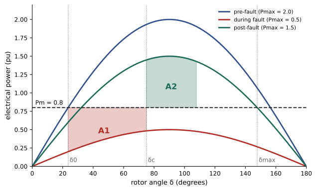
For a single machine connected to a large system (an infinite bus) through a reactance \(X\), electrical output is \(P_e = P_{\max}\sin\delta\) with \(P_{\max} = E'V/X\), using the voltage behind transient reactance (Lesson 3). The value of \(P_{\max}\) depends on the network state: it falls sharply during a fault (to zero for a three-phase fault at the generator terminals) and, after the faulted line is removed, recovers to a value lower than before because the remaining network has a higher reactance.

Multiplying the swing equation (without damping) by \(d\delta/dt\) and integrating shows that the rotor stops accelerating relative to the system, and reaches its maximum angle, when the energy gained during acceleration equals the energy given back during deceleration. On the power-angle diagram these energies are areas, which gives the equal-area criterion:

• The accelerating area \(A_1\) lies between the \(P_m\) line and the fault-on curve, from the initial angle \(\delta_0\) to the clearing angle \(\delta_c\).
• The decelerating area \(A_2\) lies between the post-fault curve and the \(P_m\) line, from \(\delta_c\) to the maximum angle.
• The system is stable if the available decelerating area, up to the angle \(\delta_{\max} = \pi - \arcsin(P_m/P_{\max,\text{post}})\) where the post-fault curve falls below \(P_m\) again, is at least \(A_1\).

Setting the two areas equal at the limit gives the critical clearing angle \(\delta_{cr}\):

For a fault that reduces output to zero, the angle grows as \(\delta = \delta_0 + \tfrac12(\omega_s P_m/2H)t^2\), so the critical clearing time follows directly. Otherwise it is found by numerically integrating the swing equation.

import numpy as np

# Single machine, infinite bus: Pmax before, during and after a fault (pu), H in seconds, 60 Hz
H, f0, Pm = 5.0, 60.0, 0.8
P_pre, P_fault, P_post = 2.0, 0.5, 1.5
d0 = np.arcsin(Pm / P_pre)

def simulate(t_clear, t_end=3.0, dt=0.0005):
    d, w, t = d0, 0.0, 0.0                              # w = speed deviation in rad/s
    dmax = d
    while t < t_end:
        Pe = (P_fault if t < t_clear else P_post) * np.sin(d)
        dw = np.pi * f0 / H * (Pm - Pe)                 # swing equation: (2H / w_s) d2delta/dt2 = Pm - Pe
        w += dw * dt; d += w * dt; t += dt
        dmax = max(dmax, d)
        if d > np.pi: return False, dmax
    return True, dmax

for tc in (0.10, 0.20, 0.30, 0.34, 0.35, 0.40):
    ok, dmax = simulate(tc)
    result = "stable" if ok else "loses synchronism"
    print(f"clearing at {tc * 1000:4.0f} ms: {result}; maximum angle {np.degrees(min(dmax, np.pi)):5.1f} deg")

# Equal-area criterion for the critical clearing angle
dmax_post = np.pi - np.arcsin(Pm / P_post)
cos_dc = (Pm * (dmax_post - d0) + P_post * np.cos(dmax_post) - P_fault * np.cos(d0)) / (P_post - P_fault)
dc = np.arccos(cos_dc)
lo, hi = 0.0, 1.0                                       # find the clearing time that reaches dc by bisection
for _ in range(40):
    mid = (lo + hi) / 2
    ok, _ = simulate(mid)
    lo, hi = (mid, hi) if ok else (lo, mid)
print(f"initial angle {np.degrees(d0):.1f} deg; critical clearing angle {np.degrees(dc):.1f} deg; critical clearing time about {lo * 1000:.0f} ms")

clearing at  100 ms: stable; maximum angle  51.4 deg
clearing at  200 ms: stable; maximum angle  73.2 deg
clearing at  300 ms: stable; maximum angle 108.6 deg
clearing at  340 ms: stable; maximum angle 137.5 deg
clearing at  350 ms: loses synchronism; maximum angle 180.0 deg
clearing at  400 ms: loses synchronism; maximum angle 180.0 deg
initial angle 23.6 deg; critical clearing angle 89.6 deg; critical clearing time about 343 ms

Clearing at 340 ms survives with the angle peaking at 137.5°, close to the 148° limit; clearing 10 ms later loses synchronism. The equal-area criterion gives the critical clearing angle (89.6°), and the simulation converts it to time. Note how the maximum angle grows faster and faster as clearing is delayed: stability margins disappear abruptly rather than gradually.

Multi-machine transient stability

Real systems have hundreds of generators, each with its own swing equation, coupled through the network. Transient stability programs integrate these differential equations together with the algebraic network equations, using detailed models of generators (with transient and subtransient effects), excitation systems, governors, loads, protection and, increasingly, inverter-based resources. Studies simulate a list of credible contingencies, typically faults on each line cleared by normal protection and by backup protection, and check that all machines remain in synchronism, that oscillations are damped, and that voltages recover within criteria. Transmission planners run thousands of such simulations to set operating limits on key interfaces.

A useful insight from multi-machine studies is that instability usually appears as one machine or a group of machines swinging apart from the rest. Machines close to the fault, with low inertia or heavily loaded, are the most vulnerable. Transmission corridors linking generation-rich and load-rich regions often have their transfer limits set by transient stability rather than by thermal ratings.

Small-signal stability

Even without large disturbances, a power system continuously experiences small changes in load and generation, and it must damp the resulting oscillations. Linearizing the swing equation around an operating point gives a second-order system:

The synchronizing coefficient \(K_s\) is the slope of the power-angle curve; it must be positive (\(\delta_0 < 90°\)) for the machine to be pulled back. The natural frequency of rotor oscillation is

Electromechanical oscillations fall into several types:

• Local modes, 0.7 to 2 Hz: one plant against the rest of the system.
• Inter-area modes, 0.1 to 0.8 Hz: groups of generators in one region swinging against groups in another, across weak interconnections. They are the hardest to damp; the western North American interconnection has well-known modes near 0.25 and 0.4 Hz.
• Control and torsional modes, involving excitation controls and the shaft systems of turbine generators.

Fast-acting voltage regulators, essential for transient stability, tend to reduce the damping of these modes, sometimes making it negative. The 1996 western North American blackout involved growing inter-area oscillations. The cure is the power system stabilizer (Lesson 3), which modulates excitation in phase with speed deviations to add damping torque. Small-signal stability is analyzed by computing the eigenvalues of the linearized multi-machine model: each complex pair gives a mode's frequency and damping ratio, and planners typically require damping ratios of at least 3% to 5%. Wide-area measurement systems using synchronized phasor measurement units (PMUs) now monitor these oscillations in real time.

Improving stability

Transient stability improves when the accelerating area shrinks or the decelerating area grows:

• Faster fault clearing: high-speed protection and breakers (2-cycle breakers on critical lines) reduce the accelerating area directly.
• Single-pole tripping and reclosing: most faults involve one phase, and tripping only that phase keeps power flowing on the other two.
• Higher system voltage, parallel lines and series compensation increase \(P_{\max}\).
• Fast excitation with high ceiling voltage boosts \(E\) during and after the fault.
• Fast valving, which briefly reduces turbine power, and braking resistors, which absorb surplus power, reduce acceleration.
• Special protection (remedial action) schemes trip generators or shed load automatically for specified contingencies, preserving the rest of the system.
• Controlled separation (islanding) splits the system along planned boundaries when loss of synchronism cannot be prevented, with out-of-step relays detecting the condition.

Inverter-based resources change the picture. They have no inherent inertia, so lower system inertia means faster frequency changes and larger angle swings for the same disturbance, but their controls can respond far faster than any turbine. Grid-following inverters can lose synchronism with a weak grid through their phase-locked loops; grid-forming inverters behave more like voltage sources and can provide synthetic inertia and damping. Stability studies of systems with high inverter penetration increasingly need electromagnetic transient (EMT) simulation, which models the converters' fast controls in detail, rather than traditional phasor-based programs.