
ELE-380 · Lesson 5 of 12 · 27 min
Reactive power, voltage control and voltage stability
Frequency is a single quantity shared by the whole interconnection, but voltage is local: it varies from bus to bus, and it is governed largely by the flow of reactive power. Too little reactive support and voltages sag, motors stall, and in the worst case voltage collapses across a region, as it did in several major blackouts. Too much and voltages rise above equipment ratings. This lesson explains why reactive power and voltage are linked, describes the devices that produce, absorb and control reactive power, introduces tap-changing transformers and their interaction with loads, and studies voltage stability with PV and QV curves.
Why voltage follows reactive power
Consider power flowing over a line of reactance \(X\) from a sending bus at voltage \(V_S\) to a receiving bus at \(V_R\). The voltage drop along the line is approximately
At transmission level \(X\) is typically five to ten times \(R\), so the drop depends far more on reactive than on real power. Transferring reactive power over long distances is therefore inefficient: it causes large voltage drops and \(I^2R\) losses, while the real power carried is unchanged. The practical rule is that reactive power should be supplied close to where it is consumed. This also explains the decoupling exploited in load flow (Lesson 6): real power is tied to voltage angles and reactive power to voltage magnitudes.
Worked problem
Voltage drop from real and reactive flow
A 138 kV line has \(R = 0.02\) pu and \(X = 0.10\) pu on 100 MVA. It delivers 80 MW and 40 Mvar to a bus at 1.0 pu. Estimate the voltage drop and the share due to reactive power.
Show solution
- \(\Delta V \approx 0.02 \times 0.8 + 0.10 \times 0.4 = 0.016 + 0.040 = 0.056\) pu.
- Reactive share: \(0.040/0.056 = 71\%\).
Answer: About 5.6% drop, 71% of it caused by the 40 Mvar of reactive flow. Supplying the 40 Mvar locally with a capacitor bank would cut the drop to about 1.6%.
Sources and sinks of reactive power
Every element of the system produces or consumes reactive power:
- Loads: induction motors, transformers and many electronic loads absorb reactive power. Lagging power factors of 0.85 to 0.95 are typical.
- Transmission lines produce reactive power through their shunt capacitance (\(V^2 B\)) and absorb it in their series reactance (\(I^2 X\)). Below surge impedance loading a line is a net source, above it a net sink (Lesson 4).
- Cables have large capacitance and are strong sources, which limits the length of AC cable circuits.
- Transformers absorb reactive power in their leakage reactance, roughly 5% to 15% of their loading squared.
- Generators supply or absorb reactive power within their capability curves (Lesson 3).
The balance shifts over the day. At peak load, heavily loaded lines and motor loads absorb large amounts of reactive power and voltages tend to sag. At light load, line charging dominates and voltages rise; operators then switch off capacitors, switch in reactors and run generators underexcited.
Reactive power control devices
| Device | How it works | Speed | Notes |
|---|---|---|---|
| Shunt capacitor bank | supplies \(Q = V^2\omega C\) when switched in | seconds to minutes (mechanically switched) | cheap; output falls with the square of voltage |
| Shunt reactor | absorbs \(Q = V^2/\omega L\) | switched | controls high voltage on long lines and cables |
| Series capacitor | cancels part of a line's reactance | fixed or switched | raises transfer capability; self-regulating |
| Synchronous condenser | synchronous machine with controllable excitation | continuous, fast | adds inertia and fault current; output holds up at low voltage |
| Static var compensator (SVC) | thyristor-switched capacitors and controlled reactors | one to two cycles | output falls with voltage squared like a capacitor |
| STATCOM | voltage-source converter injecting controllable current | within a cycle | output current held at low voltage, so Q falls only linearly |
| Inverter-based resources | wind, solar and batteries controlling Q within their current rating | fast | required by grid codes to provide voltage support |
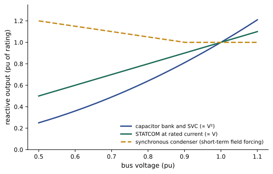
The behavior at low voltage matters most in emergencies. A capacitor bank rated 100 Mvar at 1.0 pu supplies only 81 Mvar at 0.9 pu and 64 Mvar at 0.8 pu, just when support is most needed. A STATCOM holding rated current supplies 90 and 80 Mvar at the same voltages, and a synchronous condenser can briefly exceed its rating. That is why dynamic reactive devices are placed where voltage collapse is a risk, while cheaper switched capacitors provide the bulk of steady-state support.
Tap-changing transformers
Transformers with tap changers adjust their turns ratio to regulate voltage. Off-load tap changers, set during outages, compensate for seasonal or permanent differences. On-load tap changers (OLTCs) change taps under load in steps of about 0.625% to 1.25%, over a range of typically ±10%, controlled automatically to hold the secondary voltage within a band. Each operation takes a few seconds, with intentional time delays of 30 to 60 seconds to avoid hunting and wear.
A tap changer does not create reactive power; it redistributes it. Raising the secondary voltage of a distribution transformer draws more reactive power from the transmission system, lowering the primary voltage. In a weak system this can make things worse, as explained below. Coordination matters too: transformers in series should operate with progressively longer time delays from the transmission level downward, so the upstream tap changers act first.
Worked problem
Tap setting to restore voltage
A 138/25 kV transformer with an OLTC has its secondary voltage at 0.95 pu under peak load with the tap at nominal. The tap changer moves in steps of 0.625% of the primary-side ratio. How many steps are needed to bring the secondary above 0.99 pu, assuming the primary voltage stays fixed?
Show solution
- Required rise: \(0.99/0.95 = 1.042\), about 4.2%.
- Steps: \(4.2/0.625 = 6.7\), so 7 steps (4.375%), giving \(0.95 \times 1.04375 = 0.992\) pu.
Answer: Seven steps, about 3.5 to 7 minutes with typical delays. In reality the primary voltage falls slightly as the load draws more reactive power, so an additional step may be needed.
Voltage stability and PV curves
Voltage stability is the ability of a system to maintain acceptable voltages at all buses after a disturbance. Its limit is easiest to see in a two-bus system: a source behind a line of reactance \(X\) supplying a load \(P + jQ\). Solving for the receiving voltage gives a quadratic in \(V^2\):
For each load level there are two solutions, a high-voltage one (the normal operating point) and a low-voltage one (high current, unstable under most load characteristics). As the load increases, the two meet at the nose of the PV curve, the maximum power that can be delivered. Beyond it there is no solution: voltage collapses. For unity power factor, the maximum is \(P_{\max} = E^2/(2X)\) at \(V = E/\sqrt2\).
import numpy as np

# Two-bus system: source 1.0 pu behind a line of reactance X feeding a load at power factor pf
X = 0.5
def nose(pf, Bc=0.0):
    tanphi = np.tan(np.arccos(pf))
    best = (0, None)
    pts = []
    for P in np.linspace(0, 2.0, 20001):
        Q = P * tanphi
        # receiving-end voltage from V^4 + (2QX - E^2) V^2 + X^2 (P^2 + Q^2) = 0, with shunt capacitor Bc
        Qn = Q - Bc                                    # capacitor supplies Bc * V^2, approximated at V = 1
        b = 2 * Qn * X - 1.0
        disc = b ** 2 - 4 * X ** 2 * (P ** 2 + Qn ** 2)
        if disc < 0:
            break
        V2 = (-b + np.sqrt(disc)) / 2
        best = (P, np.sqrt(V2))
        pts.append((P, np.sqrt(V2)))
    return best, pts

for pf, Bc, label in ((0.9, 0, "pf 0.90 lagging"), (1.0, 0, "unity pf"), (0.9, 0.4, "pf 0.90 with 0.4 pu capacitor")):
    (Pmax, Vnose), pts = nose(pf, Bc)
    v_at_06 = [v for p, v in pts if p >= 0.6][0]
print(f"{label:30s}: maximum load {Pmax:.3f} pu at V = {Vnose:.3f} pu; voltage at P = 0.6: {v_at_06:.3f} pu")pf 0.90 lagging : maximum load 0.627 pu at V = 0.596 pu; voltage at P = 0.6: 0.690 pu unity pf : maximum load 1.000 pu at V = 0.707 pu; voltage at P = 0.6: 0.949 pu pf 0.90 with 0.4 pu capacitor : maximum load 0.942 pu at V = 0.692 pu; voltage at P = 0.6: 1.009 pu
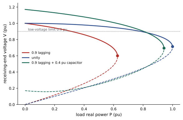
The results show three lessons. Lagging reactive demand sharply reduces the deliverable power, here from 1.0 to 0.63 pu. Compensation restores most of it. But with compensation, the voltage at a given load looks healthy, near 1.0 pu, right up to a point not far from the nose: voltage magnitude alone is a poor indicator of the distance to collapse. (The calculation also treats the capacitor as constant reactive power; a real capacitor's output falls with voltage, which makes the true nose lower and steeper.) Operators therefore monitor margins in megawatts: how much more load or transfer the system can take before reaching the nose, typically requiring at least 5% margin after the worst contingency.
QV curves and reactive margin
A complementary tool is the QV curve: at a chosen bus, plot the reactive power a fictitious compensator would need to inject to hold each voltage, keeping loads and generation fixed. The bottom of the curve gives the reactive power margin: if the minimum lies below zero, the bus has spare reactive capability equal to its depth; if above zero, no operating point exists without added reactive support. QV curves are computed bus by bus with repeated load flows and identify the weakest buses where compensation is most effective.
Sensitivity offers a quick indicator. Near the nose, \(dV/dQ\) at the weak bus becomes large and then changes sign: injecting reactive power, which normally raises voltage, starts to lower it. Modal analysis of the reduced load flow Jacobian (the smallest eigenvalue of the \(\partial Q/\partial V\) relation) identifies the buses participating in the most critical mode.
Mechanisms of voltage collapse
Voltage collapse usually unfolds over tens of seconds to minutes, through the interaction of loads, tap changers and generator limiters:
- A contingency, such as a line or generator outage, increases the reactance between sources and loads, reducing the maximum transfer.
- Voltage drops; load power briefly falls, because many loads behave partly like impedances.
- OLTCs at load buses raise the secondary voltage over the next minute, restoring load power, which draws more current through the weakened network and pulls transmission voltages down further.
- Generators supplying more reactive power reach their field current limits; overexcitation limiters cut them back after a time delay, and their buses lose voltage control.
- Induction motors slow down and draw more reactive current; air conditioner compressors may stall, drawing several times their normal current until thermal protection trips them.
The cycle can end in a cascade of protective tripping and a blackout. The 2003 Northeast blackout in North America and several European events involved voltage problems combined with line overloads. Fault-induced delayed voltage recovery, in which stalled residential air conditioners hold voltage low for several seconds after a fault is cleared, is a known risk in hot climates.
Countermeasures include: maintaining dynamic reactive reserves in generators, condensers and STATCOMs; switching capacitors automatically on low voltage; blocking or reversing tap changers during emergencies; secondary voltage control that coordinates generators across a region; and, as a last resort, undervoltage load shedding, which drops blocks of load when voltage stays low for several seconds, sacrificing some customers to save the system.
Common mistakes
MistakeTransporting large amounts of reactive power over long lines.
InsteadSupply reactive power close to where it is consumed.
MistakeJudging the distance to voltage collapse by the voltage magnitude.
InsteadWith compensation, voltage can look normal near the nose; monitor megawatt and reactive margins.
MistakeRelying only on capacitor banks for emergency voltage support.
InsteadTheir output falls with voltage squared; place dynamic devices where collapse is a risk.
MistakeAssuming tap changers always help voltage.
InsteadThey restore load and can accelerate collapse in a weak system; block them in emergencies.
MistakeIgnoring generator reactive limits in voltage studies.
InsteadModel field limits and limiter time delays; they often trigger collapse.
Summary and key terms
- At transmission level voltage drop depends mainly on reactive flow, so reactive power should be supplied locally.
- Loads, lines, cables, transformers and generators each produce or absorb reactive power, and the balance changes with load.
- Capacitors, reactors, condensers, SVCs, STATCOMs and inverter resources control reactive power, with very different low-voltage behavior.
- On-load tap changers regulate voltage by redistributing reactive power and must be coordinated.
- PV curves show the maximum transfer at the nose; QV curves show reactive margins at weak buses.
- Voltage collapse develops through load restoration, tap changers and generator limiters; reserves, coordination and load shedding prevent it.
- Reactive power
- The oscillating component of power that sustains electric and magnetic fields.
- Shunt capacitor
- A capacitor bank connected line to ground or line to line to supply reactive power.
- Shunt reactor
- An inductor that absorbs reactive power to limit high voltage.
- STATCOM
- A converter-based static compensator injecting controllable reactive current.
- SVC
- A static var compensator using thyristor-controlled reactors and capacitors.
- On-load tap changer
- A transformer mechanism that changes the turns ratio while energized.
- Voltage stability
- The ability to maintain acceptable voltages at all buses after disturbances.
- PV curve
- A plot of bus voltage against load or transfer, showing the nose point.
- QV curve
- A plot of reactive injection needed against bus voltage, showing reactive margin.
- Undervoltage load shedding
- Automatic disconnection of load when voltage remains low.
Practice problems
Work each problem on paper first, then reveal the answer to check.
\(R = 0.01\), \(X = 0.08\), \(P = 1.0\), \(Q = 0.5\) at \(V = 1\): approximate drop?
Show answer
\(0.01 + 0.04 = 0.05\) pu.
Output of a 50 Mvar capacitor at 0.85 pu voltage?
Show answer
\(50 \times 0.7225 = 36\) Mvar.
Output of a 50 Mvar STATCOM at rated current and 0.85 pu?
Show answer
42.5 Mvar.
Maximum unity-power-factor load for \(E = 1.0\), \(X = 0.25\)?
Show answer
\(1/(2 \times 0.25) = 2.0\) pu.
Voltage at the nose for unity power factor with \(E = 1.05\)?
Show answer
\(1.05/\sqrt2 = 0.742\) pu.
Number of 0.625% steps to raise voltage by 3%?
Show answer
5 steps (3.125%).
Why are tap changers in series given increasing time delays downstream?
Show answer
So upstream changers act first and they do not hunt.
A QV curve minimum is at +20 Mvar. What does it mean?
Show answer
No operating point exists without at least 20 Mvar of added support.
Name two loads that make collapse worse.
Show answer
Tap-changer-regulated loads and stalling induction motors (air conditioners).
What is a last-resort protection against voltage collapse?
Show answer
Undervoltage load shedding.
Lesson quiz · 5 questions
Score 60% or more to complete this lesson.
Create a free account to save your progress, take quizzes and earn a certificate.