
ELE-380 · Lesson 3 of 12 · 29 min
Synchronous generators in the power system
Almost all of the world's electricity has historically come from synchronous generators driven by steam, gas and hydro turbines, and even as inverter-based wind, solar and batteries grow, synchronous machines still set the frequency, supply most of the system's inertia and fault current, and regulate voltage across much of the grid. A power systems engineer needs a model of the generator that is simple enough for network studies yet captures its limits: how much real and reactive power it can supply, how its internal voltage and load angle respond to loading, and how it behaves in the first cycles of a fault. This lesson develops the steady-state model, the power-angle relations, reactive power control, the capability curve, salient-pole effects, the transient and subtransient reactances used in fault and stability studies, excitation control, and a comparison with inverter-based resources.
Construction and operation
A synchronous generator has a three-phase armature winding on the stator and a field winding on the rotor, supplied with direct current by the excitation system. Turning the rotor makes its magnetic field rotate, inducing three-phase voltages in the stator at a frequency tied rigidly to the speed:
where \(n\) is in r/min and \(p\) is the number of poles. Steam and gas turbines run fast, so their generators have two or four poles (3,600 or 1,800 r/min at 60 Hz) and cylindrical (round) rotors able to withstand large centrifugal forces. Hydro turbines run slowly, so their generators have many poles (a 72-pole machine turns at 100 r/min) on a large-diameter salient-pole rotor. Large units are rated from a few hundred to over 1,500 MVA, at stator voltages of 13.8 to 26 kV, and are connected to the transmission system through generator step-up transformers.
When stator currents flow, they create their own rotating field, which turns in step with the rotor. The interaction of the two fields produces the torque that opposes the turbine. Because every synchronous machine on an interconnected system turns at a speed locked to the common frequency, the machines are said to be in synchronism, and keeping them so after disturbances is the stability problem of Lesson 8.
The steady-state model
For a round-rotor machine in steady state, each phase is represented by an internal voltage \(E\), proportional to field current and speed, behind the synchronous reactance \(X_s\), which accounts for both the armature reaction and leakage flux. Armature resistance is small (well under 1% on the machine base) and is usually neglected in network studies:
Synchronous reactances are large: 1.5 to 2.2 pu for round-rotor machines on their own rating, and 0.8 to 1.2 pu for salient-pole machines. The angle \(\delta\) by which \(\mathbf{E}\) leads the terminal voltage \(\mathbf{V}\) is the load angle (or power angle). It corresponds physically to the angle by which the rotor leads the rotating field set up by the network.
With \(\mathbf{V} = V\angle 0\) and \(\mathbf{E} = E\angle\delta\), the power delivered at the terminals follows from the same analysis as power flow over a reactance (Lesson 4):
Real power is controlled by the turbine: opening the steam or water valves increases mechanical torque, the rotor advances, \(\delta\) grows and electrical output rises to match. Reactive power is controlled by the field: raising the field current raises \(E\), and the machine delivers more reactive power. The maximum power at a given excitation, \(P_{\max} = EV/X_s\) at \(\delta = 90°\), is the steady-state stability limit; beyond it, more mechanical input cannot be converted to electrical output and the rotor pulls out of step.
Worked problem
Internal voltage and load angle
A generator with \(X_s = 1.8\) pu delivers 0.8 pu real power at 0.85 power factor lagging to an infinite bus at 1.0 pu. Find \(E\), \(\delta\) and the reactive power.
Show solution
- Current: \(|I| = 0.8/0.85 = 0.941\) pu at \(-31.8°\); \(\mathbf{I} = 0.80 - j0.496\) pu.
- \(\mathbf{E} = 1.0 + j1.8(0.80 - j0.496) = 1.0 + 0.893 + j1.44 = 1.893 + j1.44\).
- \(|E| = 2.38\) pu, \(\delta = 37.3°\). Reactive power: \(Q = 0.8\tan 31.8° = 0.50\) pu.
Answer: \(E = 2.38\) pu at \(37.3°\), supplying 0.50 pu of reactive power. Check: \(P = 2.38 \times 1.0/1.8 \times \sin 37.3° = 0.80\) pu.
Reactive power and excitation
At constant real power, the field current determines whether the machine produces or absorbs reactive power:
- Overexcited: \(E\cos\delta > V\), the machine supplies reactive power (lagging power factor at its terminals), supporting system voltage. Generators run this way most of the time, because loads and lines absorb reactive power.
- Normally excited: \(E\cos\delta = V\), unity power factor.
- Underexcited: \(E\cos\delta < V\), the machine absorbs reactive power (leading power factor). This is needed at night in systems with long, lightly loaded lines or cables, whose charging produces surplus reactive power and high voltages (Lesson 4).
Plotting armature current against field current at constant real power gives the V-curves: the current is lowest at unity power factor and rises on either side. Underexcitation has a price: with smaller \(E\), the load angle must be larger to deliver the same real power, so the margin to the stability limit shrinks.
import numpy as np

# Round-rotor generator on an infinite bus, per unit on the machine rating
V, Xs = 1.0, 1.8                                       # terminal voltage and synchronous reactance
for P, pf in ((0.8, 0.85), (0.8, 1.0), (0.8, 0.95)):
    lead = pf == 0.95                                  # third case: leading (absorbing vars)
    phi = np.arccos(pf) * (-1 if lead else 1)
    I = P / (V * pf) * np.exp(-1j * phi)               # lagging current for exporting vars
    E = V + 1j * Xs * I                                # internal voltage
    Q = P * np.tan(phi)
    print(f"P = {P}, Q = {Q:+.2f}: |E| = {abs(E):.2f} pu, load angle {np.degrees(np.angle(E)):5.1f} deg")

# Capability curve limits at P = 0.8: armature current limit and field limit (E max 2.6 pu)
S_max, E_max = 1.0, 2.6
Q_arm = np.sqrt(S_max ** 2 - 0.8 ** 2)
Q_field = -V ** 2 / Xs + np.sqrt((E_max * V / Xs) ** 2 - 0.8 ** 2)
print(f"at P = 0.8: armature limit Q = {Q_arm:.2f}, field limit Q = {Q_field:.2f}; available lagging Q = {min(Q_arm, Q_field):.2f}")
print(f"steady-state stability limit with E = 1.5: Pmax = {1.5 * V / Xs:.2f} pu")P = 0.8, Q = +0.50: |E| = 2.38 pu, load angle 37.3 deg P = 0.8, Q = +0.00: |E| = 1.75 pu, load angle 55.2 deg P = 0.8, Q = -0.26: |E| = 1.53 pu, load angle 69.9 deg at P = 0.8: armature limit Q = 0.60, field limit Q = 0.65; available lagging Q = 0.60 steady-state stability limit with E = 1.5: Pmax = 0.83 pu
At 0.95 leading, the internal voltage falls to 1.53 pu and the load angle rises to 70°, close to the 90° limit; the corresponding maximum power is only \(1.53/1.8 = 0.85\) pu, barely above the 0.8 pu being delivered. Any disturbance could push such a machine out of step, which is why underexcitation limiters prevent operation too far into the leading region.
The capability curve
A generator's permissible operating region in the P-Q plane is bounded by several physical limits, plotted on the capability curve supplied by the manufacturer:
- Armature (stator) heating: the stator current limit is a circle \(P^2 + Q^2 = S_{\text{rated}}^2\), centered on the origin.
- Field (rotor) heating: the maximum field current sets a maximum \(E\), and the locus of constant \(E\) is a circle centered at \((0, -V^2/X_s)\) with radius \(E_{\max}V/X_s\). It limits reactive output at lagging power factors.
- Prime mover: the turbine's maximum output caps real power, a horizontal line.
- Underexcited limits: stator end-region heating, caused by leakage flux at the ends of the core when the machine is underexcited, and the practical stability limit, a margin inside the theoretical \(\delta = 90°\) line, together bound the leading region.
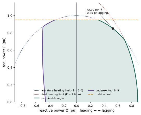
The rated power factor (typically 0.85 to 0.9 lagging) marks the corner where the armature and field limits meet. At full real power, the reactive capability is therefore limited; at reduced real power, more reactive output is available. Transmission operators specify required reactive capability in grid codes, often as a power factor range at full output (for example, 0.95 leading to 0.90 lagging) measured at the point of interconnection.
In load flow, a generator bus is a PV bus with its voltage held by the automatic voltage regulator, provided the reactive output stays within limits. When the reactive limit is reached, the bus becomes a PQ bus with Q fixed at the limit, and its voltage is no longer held (Lesson 6). Reactive limits reached by several generators at once are a classic precursor of voltage collapse (Lesson 5).
Salient-pole machines
In a salient-pole machine, the air gap is small along the axis of the poles (the direct or d-axis) and large between them (the quadrature or q-axis), so the reactance depends on the direction of the stator field. The two-reaction theory splits the armature current into d- and q-axis components with reactances \(X_d\) and \(X_q\) (with \(X_q\) typically 0.6 to 0.7 times \(X_d\)). The power-angle equation gains a second term:
The second term, the reluctance power, exists even with no field current, because the rotor tends to align its low-reluctance axis with the stator field. It makes the maximum power occur at a load angle below 90° and slightly increases it. For most network studies, a round-rotor model with \(X_s = X_d\) is an adequate approximation; stability programs use full two-axis models.
Transient and subtransient reactances
The synchronous reactance describes the machine after all magnetic transients have died away. Immediately after a sudden change such as a short circuit, the flux linking the rotor circuits cannot change instantly, because currents are induced in the field winding and in the damper (amortisseur) windings embedded in the pole faces that oppose any change. The machine therefore looks like a voltage behind a much smaller reactance, which then increases as the induced currents decay:
| Quantity | Round rotor (pu) | Salient pole (pu) | Period it describes |
|---|---|---|---|
| Subtransient reactance \(X_d''\) | 0.12 to 0.25 | 0.15 to 0.35 | first few cycles; damper currents |
| Transient reactance \(X_d'\) | 0.20 to 0.35 | 0.25 to 0.45 | about 0.1 to 2 s; field currents |
| Synchronous reactance \(X_d\) | 1.5 to 2.2 | 0.8 to 1.2 | steady state |
| Subtransient time constant \(T_d''\) | 0.02 to 0.05 s | 0.02 to 0.05 s | decay of damper currents |
| Transient time constant \(T_d'\) | 0.5 to 2 s | 1 to 3 s | decay of induced field current |
| Negative-sequence reactance \(X_2\) | about \(X_d''\) | about \((X_d'' + X_q'')/2\) | unbalanced faults |
These reactances serve different studies. Fault calculations for circuit breaker interrupting duty use \(X_d''\), which gives the highest current (Lesson 9). Transient stability studies over the first second or so model the generator as a constant voltage behind \(X_d'\) (Lesson 8). Steady-state and load flow studies use \(X_d\), or simply treat the generator as a PV source.
Worked problem
Generator fault current over time
A 500 MVA, 22 kV generator at no load and rated voltage has \(X_d'' = 0.18\), \(X_d' = 0.28\) and \(X_d = 1.9\) pu. Estimate the RMS symmetrical current for a three-phase fault at its terminals in the subtransient, transient and steady-state periods.
Show solution
- Base current: \(500 \times 10^6/(\sqrt3 \times 22{,}000) = 13.1\) kA.
- Subtransient: \(1/0.18 = 5.56\) pu, 72.9 kA. Transient: \(1/0.28 = 3.57\) pu, 46.8 kA.
- Steady state: \(1/1.9 = 0.53\) pu, 6.9 kA.
Answer: About 73 kA falling to 47 kA within a few cycles and toward 7 kA after a few seconds, ignoring the voltage regulator, which in practice boosts the field and holds the sustained current higher. The decay is why generator protection and breakers are rated on subtransient values, and why the generator decrement matters when a generator is the only source (DCE-340).
Excitation systems and control
The excitation system supplies and controls the field current. Older machines used DC exciters (a DC generator on the shaft); modern ones use static exciters, which rectify power from the generator terminals with thyristors, or brushless exciters, an inverted AC generator and rotating diode rectifier on the shaft that avoids slip rings. The automatic voltage regulator (AVR) adjusts the field to hold terminal voltage at its set point, responding within tenths of a second. Around it sit several limiters and controls:
- Overexcitation limiters protect the field winding from sustained overheating, after allowing short-term field forcing during faults.
- Underexcitation limiters keep the machine out of the unstable or end-region heating zone of the capability curve.
- Volts-per-hertz limiters prevent overfluxing of the generator and step-up transformer at low speed.
- Power system stabilizers add a damping signal based on speed or power deviations, counteracting the tendency of fast AVRs to reduce the damping of electromechanical oscillations (Lesson 8).
The turbine governor, which controls real power and responds to frequency, is the subject of Lesson 11.
Synchronous machines and inverter-based resources
Wind turbines, solar arrays and batteries connect through power electronic inverters, and their behavior differs fundamentally from that of synchronous machines:
| Property | Synchronous generator | Inverter-based resource |
|---|---|---|
| Fault current | 4 to 7 times rated, from the stored magnetic energy | limited to about 1.1 to 1.5 times rated by semiconductor ratings |
| Inertia | stored kinetic energy in the rotating mass resists frequency changes | none inherently; can be emulated by control if energy is available |
| Reactive power | set by the field; limited by the capability curve | set by control within the current limit, often very fast |
| Behavior in disturbances | determined by physics; predictable | determined by control software; varies by vendor and settings |
| Grid synchronization | electromechanical, inherent | grid-following (tracks the measured voltage) or grid-forming (creates its own voltage) |
As inverter-based resources displace synchronous machines, systems lose inertia, fault current and voltage support. Responses include synchronous condensers (synchronous machines with no turbine, run purely to supply reactive power, inertia and fault current, sometimes converted from retired generators), grid-forming inverters, and updated protection schemes. These themes return in Lessons 11 and 12.
Common mistakes
MistakeAssuming reactive power is controlled by the turbine.
InsteadReal power follows the turbine; reactive power follows the field current.
MistakeIgnoring the stability margin when running underexcited.
InsteadLower \(E\) means a larger load angle for the same power; respect underexcitation limits.
MistakeUsing synchronous reactance in fault calculations.
InsteadUse \(X_d''\) for breaker duty and \(X_d'\) for transient stability.
MistakeTreating generator reactive capability as unlimited in load flow.
InsteadConvert PV buses to PQ when they reach their reactive limits.
MistakeAssuming inverter-based resources supply fault current like generators.
InsteadInverters are current-limited to near rated current, which affects protection and voltage support.
Summary and key terms
- Synchronous generators turn at a speed locked to frequency; round rotors suit fast turbines and salient poles suit hydro.
- The steady-state model is an internal voltage behind synchronous reactance; \(P = (EV/X_s)\sin\delta\).
- The turbine controls real power and the field controls reactive power; underexcitation reduces the stability margin.
- The capability curve combines armature, field, turbine and underexcited limits.
- Subtransient, transient and synchronous reactances describe successive periods after a disturbance.
- AVRs, limiters and stabilizers control excitation; inverter-based resources differ in fault current, inertia and control.
- Synchronous reactance
- The steady-state reactance combining armature reaction and leakage.
- Load angle
- The angle by which the internal voltage leads the terminal voltage.
- Overexcited
- Operating with enough field current to supply reactive power.
- Capability curve
- The permissible region of real and reactive output of a generator.
- Reluctance power
- Power produced by saliency even without field current.
- Subtransient reactance
- The reactance in the first cycles after a disturbance, set by damper windings.
- Transient reactance
- The reactance over roughly the first second, set by the field winding.
- AVR
- Automatic voltage regulator controlling field current to hold terminal voltage.
- Power system stabilizer
- A control adding damping to electromechanical oscillations through the excitation.
- Synchronous condenser
- A synchronous machine without a prime mover, used for reactive power, inertia and fault current.
Practice problems
Work each problem on paper first, then reveal the answer to check.
Speed of a 6-pole generator at 60 Hz?
Show answer
1,200 r/min.
Poles of a hydro generator turning at 150 r/min at 60 Hz?
Show answer
48.
\(E = 2.0\), \(V = 1.0\), \(X_s = 1.6\), \(\delta = 30°\): real power?
Show answer
0.625 pu.
Reactive power for the same case?
Show answer
\((2.0 \times 0.866 - 1)/1.6 = 0.458\) pu.
Steady-state stability limit for \(E = 1.4\), \(V = 1\), \(X_s = 2\)?
Show answer
0.7 pu.
Armature limit on reactive power at \(P = 0.9\) with \(S = 1\)?
Show answer
\(\sqrt{1 - 0.81} = 0.44\) pu.
Center and radius of the field limit circle for \(E_{\max} = 2.4\), \(V = 1\), \(X_s = 2\)?
Show answer
Center \((0, -0.5)\), radius 1.2.
Subtransient fault current with \(X_d'' = 0.2\) pu at 1.0 pu voltage?
Show answer
5 pu.
Which reactance is used in transient stability studies?
Show answer
The transient reactance \(X_d'\).
Name two ways to replace the inertia and fault current lost when synchronous plants retire.
Show answer
Synchronous condensers and grid-forming inverters.
Lesson quiz · 5 questions
Score 60% or more to complete this lesson.
Create a free account to save your progress, take quizzes and earn a certificate.