
ELE-380 · Lesson 12 of 12 · 29 min
Planning, integration of new resources and a system study
The earlier lessons gave the tools of power systems analysis: per unit, generator and line models, load flow, reactive power and voltage control, economic dispatch, stability, fault analysis and frequency control. Planners combine them to decide what the system of five to fifteen years from now must look like, and to judge whether each new generator, storage plant or large load can be connected safely. This final lesson describes the planning process, resource adequacy, transmission planning standards, the interconnection of inverter-based resources and large loads, and the choice among solutions, and ends with a system study project in which you apply the course's methods to the connection of a new solar plant.
The planning process
Utilities, system operators and regulators plan the power system on several horizons. Load forecasting comes first: projections of peak demand and energy by area, built from economic growth, efficiency trends, electrification of heating and transport, and large new loads such as data centers, industrial facilities and hydrogen production. After decades of flat demand, many North American utilities now forecast strong growth, much of it from data centers, whose individual requests can exceed 1,000 MW at a single site.
Generation and transmission are then planned to meet the forecast reliably and economically. In regions with competitive markets, generation investment is largely private, guided by prices and capacity markets, while system operators plan transmission and run the interconnection process. In vertically integrated utilities, including most Canadian provincial utilities, integrated resource plans choose both. Either way, planners must answer three questions: will there be enough supply (resource adequacy), can the network deliver it reliably (transmission security), and can each new connection be accommodated (interconnection)?
Resource adequacy
Resource adequacy asks whether available generation, storage and demand response will cover load with an acceptable probability of shortfall, given forced outages, weather variability and renewable output. The traditional North American criterion is a loss of load expectation (LOLE) of 0.1 day per year, one day in ten years. Probabilistic simulations sample thousands of years of weather, load and outages to estimate LOLE and the expected unserved energy, and planners find the capacity needed to meet the criterion.
A simpler deterministic measure is the planning reserve margin, installed capacity in excess of forecast peak as a percentage of peak, typically required to be 12% to 20%. With large shares of wind, solar and storage, nameplate capacity is a poor measure of contribution, so each resource is credited with its effective load carrying capability (ELCC): the amount of additional load it allows the system to serve at the same reliability. Solar's ELCC falls as its share grows, because once solar covers midday, the risk of shortfall shifts to the evening; storage's ELCC depends on its duration relative to the length of peak periods.
Worked problem
Reserve margin with accredited capacity
A utility forecasts a peak of 10,000 MW. Its resources are 8,000 MW of thermal and hydro (accredited at 92%), 3,000 MW of solar (ELCC 15%), 2,000 MW of wind (ELCC 20%) and 1,000 MW of 4-hour storage (ELCC 85%). What is its accredited reserve margin, and does it meet a 15% requirement?
Show solution
- Accredited capacity: \(0.92 \times 8{,}000 + 0.15 \times 3{,}000 + 0.20 \times 2{,}000 + 0.85 \times 1{,}000 = 7{,}360 + 450 + 400 + 850 = 9{,}060\) MW.
- Reserve margin: \((9{,}060 - 10{,}000)/10{,}000 = -9.4\%\).
Answer: A margin of −9.4%, against a requirement of +15%: a shortfall of about 2,440 MW of accredited capacity, despite 14,000 MW of nameplate capacity. Adding more solar helps little; firm resources, longer-duration storage or demand response are needed.
Transmission planning standards
Transmission plans are tested against reliability standards. In North America, NERC TPL-001 requires planners to simulate the system for a range of conditions (peak and light load, high transfers) and contingency categories, from no contingency through single outages (N−1) to multiple and extreme events, and to show that performance meets the criteria for each:
| Category | Examples | Required performance |
|---|---|---|
| P0: system intact | normal operation | all facilities within normal ratings and voltage limits |
| P1: single contingency | loss of one line, transformer, generator or shunt device | within emergency ratings; no loss of load except radial service; stable |
| P2 to P7: multiple or complex | breaker failure, bus fault, double-circuit tower, outage overlapping maintenance | some loss of load allowed in planned amounts; no cascading |
| Extreme events | loss of a whole substation or corridor | evaluate consequences; mitigate where practical |
Each category is checked with the tools of this course: load flow and contingency analysis for thermal and voltage limits (Lessons 5 and 6), short-circuit studies for equipment duty (Lessons 9 and 10), and transient and voltage stability simulations (Lessons 5 and 8). Canadian provinces apply the NERC standards through their own regulators, and the Canadian Electricity Association and provincial operators add local criteria.
Connecting inverter-based resources
Wind, solar and battery projects wait in interconnection queues that have grown to thousands of gigawatts in North America. Each project goes through studies of increasing detail (feasibility, system impact and facilities studies, now often done in clusters) that identify the network upgrades it needs and assign their costs. Beyond thermal and voltage impacts, inverter-based resources raise specific technical questions:
- Ride-through: plants must stay connected and support the grid through voltage and frequency disturbances. IEEE 2800-2022 sets performance requirements for transmission-connected inverter-based resources, including voltage and frequency ride-through, reactive current injection during faults and fast frequency response capability. Several large events, in which hundreds of megawatts of solar tripped unexpectedly after normally cleared faults, drove these requirements.
- System strength: grid-following inverters need a stiff voltage to synchronize to. The short-circuit ratio, \(\mathrm{SCR} = S_{sc}/P_{\text{plant}}\), compares the fault level at the connection point with the plant rating; values below about 3 indicate a weak grid where controls may become unstable, requiring careful tuning, synchronous condensers or grid-forming inverters.
- Protection: low and control-dependent fault current affects the reach and selectivity of relays (Lesson 10).
- Modeling: plants must provide validated dynamic models, often including EMT models, so that studies reproduce their real behavior.
Worked problem
Short-circuit ratio
A 300 MW solar plant is proposed at a 138 kV bus where the three-phase fault level is 2,400 MVA without the plant. A nearby 200 MW wind plant connects to the same bus. Compute the plant's own SCR and a weighted SCR that considers both plants.
Show solution
- Own SCR: \(2{,}400/300 = 8.0\).
- Weighted (combined) SCR: \(2{,}400/(300 + 200) = 4.8\).
Answer: An own SCR of 8 looks strong, but the combined value of 4.8, which accounts for interactions between nearby inverter plants, is closer to the weak range. If a planned retirement of a nearby synchronous plant reduces the fault level, detailed EMT studies would be required.
Connecting large loads
Large loads raise their own planning questions. A data center campus of 500 to 2,000 MW can exceed the capacity of the local transmission network and require new lines and substations, with lead times longer than the data center's construction. Load behavior during disturbances matters too: in July 2024, a transmission fault in northern Virginia caused about 1,500 MW of data center load to transfer to backup power at once, an event that shifted the system frequency and voltage and prompted NERC to study large-load ride-through. Planners now ask large loads for ride-through characteristics, ramp rates and dynamic models, much as they do for generators, and some utilities offer faster connections to loads that accept curtailment during grid emergencies or bring their own generation and storage (DCE-340).
Choosing solutions
When studies reveal violations, there are usually several possible solutions, compared on cost, reliability, lead time and risk:
- New lines, transformers and substations: the traditional answer, durable but slow, often taking 7 to 15 years for major lines because of permitting.
- Reconductoring with advanced (high-temperature, low-sag) conductors: can double a line's capacity on existing towers within a few years.
- Grid-enhancing technologies: dynamic line ratings that use real-time weather to raise ratings when cooling is good, power flow controllers that push flow away from overloaded paths, and topology optimization that switches lines to relieve congestion.
- Storage and non-wires alternatives: batteries placed to relieve a constraint, or demand response, can defer upgrades.
- Special protection schemes that trip generation for specific contingencies, allowing higher normal transfers (Lesson 8).
Economic analysis compares the present value of costs with benefits such as reduced congestion (from production cost simulations based on Lesson 7), reduced losses and improved reliability, increasingly over many future scenarios rather than a single forecast.
System study project
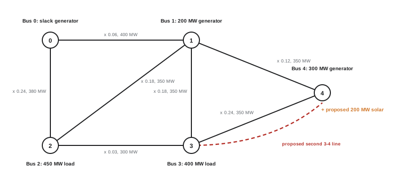
The project applies the course's methods to a planning question. A developer proposes a 200 MW solar plant at bus 4 of the five-bus 230 kV system shown in the figure. You are to determine whether the plant can connect without violating the N−1 criterion, and if not, recommend a reinforcement.
Step 1: Build and check the model
Assemble the network data in per unit (Lesson 2), check line parameters against typical values for 230 kV (Lesson 4), and solve the base case load flow (Lesson 6). Compare the results with any available measurements and confirm that voltages and flows are reasonable before studying changes.
Step 2: Steady-state contingency analysis
Solve the system intact and with each single line out, before and after adding the plant, and compare flows with ratings. The DC load flow is adequate for a first screening of thermal limits; AC load flows then check voltages and reactive power.
import numpy as np

# Five-bus DC study. Lines: (from, to, reactance pu, rating MW). Bus 0 is the slack.
lines = [(0, 1, 0.06, 400), (0, 2, 0.24, 380), (1, 2, 0.18, 350), (1, 3, 0.18, 350), (1, 4, 0.12, 350), (2, 3, 0.03, 300), (3, 4, 0.24, 350)]
P = np.array([0.0, 200.0, -450.0, -400.0, 300.0])      # injections in MW (generation positive); slack balances
P[0] = -P[1:].sum()

def dc_flows(lines, P):
    n = len(P)
    B = np.zeros((n, n))
    for i, j, x, _ in lines:
        B[i, i] += 1 / x; B[j, j] += 1 / x; B[i, j] -= 1 / x; B[j, i] -= 1 / x
    theta = np.zeros(n)
    theta[1:] = np.linalg.solve(B[1:, 1:], P[1:] / 100)          # 100 MVA base
    return [100 * (theta[i] - theta[j]) / x for i, j, x, _ in lines]

def study(lines, P, title):
    base = dc_flows(lines, P)
    print(title)
    print("  base case loading: " + ", ".join(f"{i}-{j} {abs(f) / r:.0%}" for (i, j, _, r), f in zip(lines, base)))
    worst = []
    for k, out in enumerate(lines):
        rest = lines[:k] + lines[k + 1:]
        try:
            fl = dc_flows(rest, P)
        except np.linalg.LinAlgError:
            worst.append(f"outage {out[0]}-{out[1]} islands the system"); continue
        for (i, j, _, r), f in zip(rest, fl):
            if abs(f) > r:
                worst.append(f"outage {out[0]}-{out[1]} overloads {i}-{j} at {abs(f) / r:.0%}")
    print("  N-1 violations: " + ("; ".join(worst) if worst else "none"))

study(lines, P, "Existing system")
P2 = P.copy(); P2[4] += 200; P2[0] -= 200               # add 200 MW of solar at bus 4, displacing slack generation
study(lines, P2, "With 200 MW of new solar at bus 4")
lines3 = lines + [(4, 3, 0.24, 350)]                    # reinforcement: a second line between buses 3 and 4
study(lines3, P2, "With the solar and a second 3-4 line")Existing system base case loading: 0-1 37%, 0-2 53%, 1-2 63%, 1-3 62%, 1-4 26%, 2-3 9%, 3-4 60% N-1 violations: none With 200 MW of new solar at bus 4 base case loading: 0-1 3%, 0-2 42%, 1-2 62%, 1-3 58%, 1-4 66%, 2-3 24%, 3-4 77% N-1 violations: outage 1-4 overloads 3-4 at 143%; outage 3-4 overloads 1-4 at 143% With the solar and a second 3-4 line base case loading: 0-1 3%, 0-2 37%, 1-2 52%, 1-3 46%, 1-4 37%, 2-3 43%, 3-4 53%, 4-3 53% N-1 violations: none
The existing system meets N−1. With the solar plant at full output and slack generation reduced to balance, power from bus 4 leaves mainly over lines 1-4 and 3-4, and losing either one overloads the other to 143% of its rating. A second line between buses 3 and 4 removes all violations and leaves every line below 60% in the base case. Alternatives worth evaluating include reconductoring line 3-4, a special protection scheme that curtails the solar plant if line 1-4 or 3-4 trips (cheaper but adding operational risk), or a battery at bus 4 that absorbs the surplus during contingencies.
Step 3: Short-circuit and system strength
Compute three-phase and single line-to-ground fault levels at bus 4 with and without the plant and the new line (Lessons 9 and 10), check breaker ratings, and compute the short-circuit ratio of the solar plant. Model the plant as a current-limited source contributing about 1.1 to 1.2 times its rated current, mostly positive sequence.
Step 4: Voltage and reactive power
Check that the plant can meet its reactive power requirement (for example, 0.95 leading to lagging at the point of interconnection) and that voltages remain within limits for all contingencies (Lesson 5). Determine whether switched capacitors or the plant's own inverters will provide voltage control.
Step 5: Dynamic performance
Simulate faults on lines near bus 4, cleared in normal and backup times, and confirm that existing generators remain stable (Lesson 8), that the solar plant rides through without tripping, and that frequency remains acceptable after the loss of the largest unit (Lesson 11).
Step 6: Report
Summarize the assumptions, the violations found, the alternatives considered with their costs and risks, and the recommended reinforcement, with any operating restrictions until it is built.
Every step uses methods developed in this course, and each finding feeds the next: a reinforcement chosen for thermal limits changes fault levels and stability margins, which must then be rechecked. Power systems analysis is the discipline of seeing the network as a whole, so that each new connection strengthens rather than weakens the system that everyone depends on.
Common mistakes
MistakeCounting wind and solar at nameplate capacity for adequacy.
InsteadUse ELCC or other accredited values, which fall as their shares grow.
MistakeChecking only the system-intact case.
InsteadPlanning standards require contingency analysis across categories and conditions.
MistakeJudging system strength by a single plant's SCR.
InsteadUse weighted measures when several inverter plants are electrically close.
MistakeTreating large loads as passive in planning studies.
InsteadModel their ride-through and transfer behavior; sudden load loss affects frequency and voltage.
MistakeConsidering only new lines as solutions.
InsteadCompare reconductoring, grid-enhancing technologies, storage and special protection schemes.
Summary and key terms
- Planning starts from load forecasts, now driven strongly by electrification and data centers.
- Resource adequacy uses probabilistic criteria such as LOLE and accredited capacity through ELCC.
- Transmission plans are tested against contingency categories with load flow, short-circuit and stability studies.
- Inverter-based resources need ride-through capability, adequate system strength and validated models.
- Large loads require transmission capacity and defined ride-through behavior.
- Solutions range from new lines to reconductoring, grid-enhancing technologies, storage and special protection schemes, compared economically over scenarios.
- Resource adequacy
- Having enough supply to meet demand with acceptable risk.
- LOLE
- Loss of load expectation, commonly 0.1 day per year.
- Planning reserve margin
- Capacity above forecast peak, as a percentage of peak.
- ELCC
- Effective load carrying capability, the reliability contribution of a resource.
- TPL-001
- The NERC transmission system planning performance standard.
- Interconnection queue
- The list of proposed projects awaiting connection studies.
- Short-circuit ratio
- Fault level at the connection point divided by plant rating.
- IEEE 2800
- The standard for interconnection performance of inverter-based resources on transmission systems.
- Dynamic line rating
- A line rating based on real-time weather conditions.
- Non-wires alternative
- A solution such as storage or demand response that defers network upgrades.
Practice problems
Work each problem on paper first, then reveal the answer to check.
Peak 5,000 MW, accredited capacity 5,700 MW: reserve margin?
Show answer
14%.
What LOLE criterion is traditional in North America?
Show answer
0.1 day per year.
Why does the ELCC of solar fall as its share grows?
Show answer
Risk shifts to evening hours when solar does not produce.
Accredited value of 600 MW of storage at 80% ELCC?
Show answer
480 MW.
Fault level 1,500 MVA, plant 600 MW: SCR?
Show answer
2.5, a weak grid.
What does TPL-001 category P1 cover?
Show answer
Single contingencies such as the loss of one line or generator.
Name a grid-enhancing technology.
Show answer
Dynamic line rating, power flow controllers or topology optimization.
Why must large loads have ride-through requirements?
Show answer
Sudden simultaneous load loss disturbs frequency and voltage.
In the study, why did the solar plant cause N−1 violations?
Show answer
Its output leaves bus 4 over two lines; losing one overloads the other.
Name two alternatives to a new line in the study.
Show answer
Reconductoring, a special protection scheme, or storage at bus 4.
Lesson quiz · 5 questions
Score 60% or more to complete this lesson.
Create a free account to save your progress, take quizzes and earn a certificate.