High-frequency response and the Miller effect

Electronics I ended with first estimates of an amplifier's upper corner frequency. This lesson makes those estimates systematic. At high frequencies, the charge stored in a transistor's junctions and the capacitance of its load start to carry signal current, and the gain falls. Some of those capacitances are harmless; one, the capacitance between input and output of an inverting stage, is multiplied by the stage's gain and usually dominates. The tools here are the high-frequency hybrid-π model, the transition frequency f_T, Miller's theorem, the exact two-pole analysis of the common-emitter stage, and the open-circuit time-constant method, which gives a good estimate of f_H for circuits too complicated to solve by hand.

For the APS-2, the upper corner matters even though the product handles only voice frequencies. Maintenance crews carry two-way radios, an AM broadcast transmitter stands a few kilometers from one of the test intersections, and the controller cabinet holds a cellular modem. An amplifier with gain at those radio frequencies can rectify the interference and produce audible buzz or a false noise reading. Knowing where the gain really falls, and why, tells Amara where to add filtering and which stages need it.

The high-frequency transistor model

The hybrid-π model gains two capacitors at high frequencies. C_π, from base to emitter, is mostly the diffusion capacitance of the forward-biased emitter junction and grows in proportion to the collector current; a small-signal transistor at 1 mA might have 10 to 20 pF. C_μ, from base to collector, is the depletion capacitance of the reverse-biased collector junction, typically 1 to 4 pF, falling slowly as V_CB rises. MOSFETs have the corresponding C_gs and C_gd, plus drain-to-body and source-to-body junction capacitances. The transistor's own speed is summarized by its transition frequency, the frequency at which the short-circuit current gain h_fe falls to 1:

The current gain is flat at β_0 up to f_β and then falls at 20 dB per decade, reaching 1 at f_T. A small-signal transistor with f_T = 300 MHz and β_0 = 150 has f_β of only 2 MHz: above that frequency its current gain is already falling. Since C_π grows with current while g_m grows in proportion, f_T is nearly constant over the middle of a transistor's current range, falling at low currents, where junction capacitances dominate, and at high currents, where high-injection effects set in.

Miller's theorem

Consider an impedance Z connected between two nodes of a circuit whose voltages are related by a gain K, so v_2 = Kv_1. The current through Z is (v_1 − v_2)/Z = v_1(1 − K)/Z. Seen from node 1, Z behaves like an impedance Z/(1 − K) to ground; seen from node 2, like Z/(1 − 1/K). For a capacitor C and an inverting gain K = −A, this gives the Miller capacitances

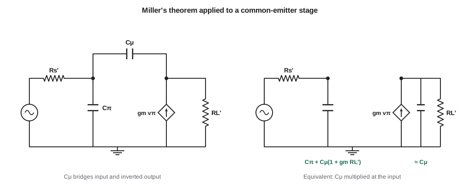
Miller's theorem is exact if K is known at the frequency of interest, but K itself changes with frequency once the capacitances act, so the usual approximation uses the mid-band gain. It works well when the input pole is far below the output pole, which is the normal case for a common-emitter stage driven from a significant source resistance. For the CE stage with the base node seeing a resistance R_s' (the source resistance in parallel with the bias network and r_π):

The exact two-pole response of the CE stage

Solving the CE small-signal circuit with C_π, C_μ and a load capacitance C_L gives a transfer function with two poles and one zero:

The zero at g_m/C_μ lies in the right half of the s-plane: at very high frequency, signal can pass forward through C_μ faster than the transistor can respond. It is normally far above f_T and harmless in a single stage, but it matters inside op amps, as lesson 4 noted. When the two poles are widely separated, the lower one is close to 1/(2πb_1), which leads directly to the time-constant method below.

Open-circuit time constants

For circuits with many capacitors, the open-circuit time-constant (OCTC) method estimates f_H without solving the full circuit. Take each capacitor in turn, with every other capacitor removed (open-circuited) and the signal source set to zero; find the resistance R_k seen by that capacitor; and add up the time constants. The sum equals the b_1 coefficient of the denominator, so if one pole dominates,

For the CE stage, C_π sees R_s', C_L sees R_L', and C_μ sees R_s'(1 + g_m R_L') + R_L', the bridging-resistance formula that every analog designer eventually knows by heart. The method is always conservative: it gives an f_H at or below the true value. It also tells the designer which capacitor to attack, because the largest R_kC_k product is the bottleneck. In the example, the C_μ term contributes 290 ns of the 327 ns, so the stage's bandwidth is a Miller problem, not a transistor-speed problem. The low-frequency counterpart, the short-circuit time-constant method from Electronics I, works the same way with capacitors shorted instead of opened.

import math
VT = 0.02585
IC, beta = 1e-3, 100
Cpi, Cmu, CL = 16e-12, 2e-12, 5e-12
Rsig_bias, RL = 1e3, 5e3
gm = IC / VT; rpi = beta / gm
Rs = Rsig_bias * rpi / (Rsig_bias + rpi)
AM = -gm * RL * rpi / (rpi + Rsig_bias)
fT = gm / (2 * math.pi * (Cpi + Cmu))
print(f"gm = {gm*1e3:.1f} mS, rpi = {rpi:.0f} ohm, Rs' = {Rs:.0f} ohm, AM = {AM:.1f}, fT = {fT/1e6:.0f} MHz")
# Miller estimate (input pole only)
Cin = Cpi + Cmu * (1 + gm * RL)
print(f"Miller: Cin = {Cin*1e12:.0f} pF, fH = {1/(2*math.pi*Rs*Cin)/1e3:.0f} kHz")
# Open-circuit time constants
taus = {"C_pi": Rs * Cpi, "C_mu": (Rs * (1 + gm * RL) + RL) * Cmu, "C_L": RL * CL}
for k, t in taus.items():
    print(f"  tau({k:4s}) = {t*1e9:6.1f} ns")
b1 = sum(taus.values())
print(f"OCTC: b1 = {b1*1e9:.0f} ns, fH = {1/(2*math.pi*b1)/1e3:.0f} kHz")
# Exact poles of 1 + b1 s + b2 s^2
b2 = Rs * RL * (Cpi * Cmu + Cpi * CL + Cmu * CL)
disc = math.sqrt(b1 ** 2 - 4 * b2)
p1, p2 = (b1 - disc) / (2 * b2), (b1 + disc) / (2 * b2)
print(f"exact: p1 = {p1/(2*math.pi)/1e3:.0f} kHz, p2 = {p2/(2*math.pi)/1e6:.0f} MHz, zero = {gm/Cmu/(2*math.pi)/1e9:.2f} GHz")
# Gain-bandwidth product of the stage
print(f"|AM| x fH = {abs(AM)*p1/(2*math.pi)/1e6:.0f} MHz")

gm = 38.7 mS, rpi = 2585 ohm, Rs' = 721 ohm, AM = -139.5, fT = 342 MHz
Miller: Cin = 405 pF, fH = 545 kHz
  tau(C_pi) =   11.5 ns
  tau(C_mu) =  290.4 ns
  tau(C_L ) =   25.0 ns
OCTC: b1 = 327 ns, fH = 487 kHz
exact: p1 = 489 kHz, p2 = 118 MHz, zero = 3.08 GHz
|AM| x fH = 68 MHz

The exact dominant pole is about 489 kHz, within half a percent of the time-constant estimate, and the second pole is far away, above 100 MHz, which is why the estimate works. The stage's gain-bandwidth product, about 68 MHz, is only a fifth of f_T: the Miller multiplication of C_μ, not the transistor, limits the stage. Two remedies follow directly from the formula for R_μ: reduce the source resistance R_s', or reduce the gain from base to collector. Lesson 6 develops the second remedy into the cascode.

Common-base and common-collector stages

The other two configurations avoid the Miller effect. In the common-base stage, the base is grounded, so C_μ connects the output to ground and is not multiplied, and C_π sits across the low resistance looking into the emitter, about r_e. The CB stage's input pole is therefore at a very high frequency, near f_T, and its output pole is set by R_L'(C_μ + C_L). It is the natural stage for wideband current buffering.

The emitter follower is also wideband: its gain is near 1, so C_π, which connects input to output, is reduced rather than multiplied, appearing at the input as about C_π/(1 + g_m R_L'). Its upper corner is often near f_T divided by a small factor. The follower has one well-known quirk: at high frequencies its output impedance rises with frequency when driven from a large source resistance, so it looks inductive. Driving a capacitive load, such as a long cable, it can then ring or even oscillate, a problem cured with a small resistor of tens of ohms in series with the base or the output.

MOSFET stages at high frequency

The same analysis applies to MOSFETs with C_gs for C_π, C_gd for C_μ and r_π infinite. A MOSFET's f_T is g_m/(2π(C_gs + C_gd)); for modern short-channel processes it reaches tens to hundreds of gigahertz, while for discrete power MOSFETs, with gate charges of tens of nanocoulombs, the capacitances are hundreds to thousands of picofarads. The Miller effect in a power MOSFET is the Miller plateau of switching circuits: during a transition, the gate driver must supply the charge for C_gd while the drain voltage swings through the whole supply voltage, and the gate voltage sits flat until it is done.