
ECON-101 · Lesson 8 of 12 · 27 min
Production and costs
Behind every supply curve are firms deciding how much to produce. Those decisions depend on costs, and costs depend on how inputs are turned into outputs. This lesson develops the economist's theory of production and cost, which underlies the analysis of market structures in lessons 9 to 11. It introduces the distinction between the short run and the long run, the law of diminishing returns, the family of cost curves that economists use, and the idea of economies of scale. BUS-110 lesson 3 used fixed and variable costs to calculate break-even points for a business; here we look at how costs change with output and why, and we define costs in the economist's way, including opportunity costs.
Economic profit and accounting profit
Accountants measure profit as total revenue minus explicit costs, the payments a firm actually makes for wages, materials, rent and interest. Economists measure economic profit as total revenue minus all costs, including implicit costs, the opportunity costs of resources the firm uses without paying for them directly. The main implicit costs are the owner's time, which could have earned a salary elsewhere, and the owner's capital, which could have earned a return elsewhere. Economic profit is therefore smaller than accounting profit. A firm earning zero economic profit is earning a normal profit: just enough to keep its resources in their current use, because it covers all opportunity costs.
Worked problem
Accounting versus economic profit
Priya runs a bakery. Revenue last year was $410,000; wages, flour, rent and other explicit costs were $330,000. She could earn $65,000 a year as a pastry chef elsewhere, and the $100,000 of savings invested in the bakery could earn 5 % in a low-risk fund. Calculate accounting and economic profit.
Show solution
- Accounting profit = $410,000 − $330,000 = $80,000.
- Implicit costs = $65,000 forgone salary + 5 % × $100,000 = $70,000.
- Economic profit = $80,000 − $70,000 = $10,000.
Answer: The bakery earns an accounting profit of $80,000 but an economic profit of only $10,000. It is still worth running, because it earns more than Priya's best alternative, but much less than the accounting figure suggests.
The short run and the long run
Economists distinguish two time horizons. In the short run, at least one input is fixed. A factory's building and major machinery cannot be changed quickly, so in the short run the firm varies output by changing variable inputs such as labor, materials and energy. In the long run, all inputs are variable: the firm can build a new plant, close an existing one, or enter or leave the industry. The length of the short run varies by industry: a food truck can double its capacity in weeks, while a pulp mill or an oil sands project may take years.
Production and diminishing returns
A production function shows the relationship between the quantities of inputs used and the maximum output that can be produced. In the short run, with capital fixed, we can ask how output changes as more workers are added. The marginal product of labor is the extra output produced by one more worker. At first, marginal product may rise, as workers specialize and use the equipment more fully. Eventually, however, the law of diminishing marginal returns sets in: as more and more of a variable input is added to a fixed input, the marginal product of the variable input eventually declines. Picture a small kitchen with two ovens. The second and third cooks greatly increase output; the sixth and seventh mostly get in each other's way.
| Workers | Total output (pizzas per day) | Marginal product | Average product |
|---|---|---|---|
| 0 | 0 | — | — |
| 1 | 40 | 40 | 40.0 |
| 2 | 100 | 60 | 50.0 |
| 3 | 150 | 50 | 50.0 |
| 4 | 185 | 35 | 46.3 |
| 5 | 210 | 25 | 42.0 |
| 6 | 225 | 15 | 37.5 |
| 7 | 230 | 5 | 32.9 |
Diminishing returns is a short-run concept; it arises because one input is fixed. It is not the same as decreasing returns to scale, a long-run concept discussed below. Diminishing returns is one of the most reliable regularities in economics and is the reason short-run cost curves eventually slope upward.
Costs in the short run
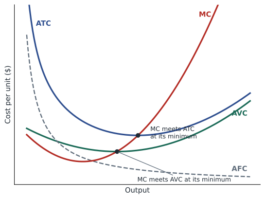
Short-run costs divide into fixed costs (FC), which do not vary with output, such as rent, insurance and the cost of equipment, and variable costs (VC), which do, such as wages, ingredients and energy. Total cost (TC) is their sum. Dividing by output gives average fixed cost (AFC), average variable cost (AVC) and average total cost (ATC). Marginal cost (MC) is the change in total cost from producing one more unit, which equals the change in variable cost because fixed cost does not change.
Marginal cost is closely linked to marginal product. If each worker costs the same wage, then when marginal product is rising, each extra pizza requires less extra labor, so marginal cost falls; when marginal product is falling, each extra pizza requires more labor, so marginal cost rises. Diminishing marginal returns therefore produces rising marginal cost.
# Short-run cost table for the pizza kitchen: fixed cost $400/day, wage $160/day per worker
fixed, wage = 400, 160
output = [0, 40, 100, 150, 185, 210, 225, 230]
print("workers   Q    VC    TC    AFC    AVC    ATC     MC")
for w, q in enumerate(output):
    vc = wage * w
    tc = fixed + vc
    if q == 0:
        print(f"{w:7} {q:4} {vc:5} {tc:5}")
        continue
    mc = (tc - (fixed + wage * (w - 1))) / (q - output[w - 1])
print(f"{w:7} {q:4} {vc:5} {tc:5} {fixed / q:6.2f} {vc / q:6.2f} {tc / q:6.2f} {mc:6.2f}")workers Q VC TC AFC AVC ATC MC
0 0 0 400
1 40 160 560 10.00 4.00 14.00 4.00
2 100 320 720 4.00 3.20 7.20 2.67
3 150 480 880 2.67 3.20 5.87 3.20
4 185 640 1040 2.16 3.46 5.62 4.57
5 210 800 1200 1.90 3.81 5.71 6.40
6 225 960 1360 1.78 4.27 6.04 10.67
7 230 1120 1520 1.74 4.87 6.61 32.00The table shows the typical patterns. Average fixed cost falls continuously as the fixed cost is spread over more output. Marginal cost falls at first, as the second worker adds 60 pizzas, and then rises steadily as diminishing returns set in, reaching $32 per pizza for the seventh worker. Average variable cost and average total cost are U-shaped. And a key relationship holds: marginal cost cuts through the minimum points of both AVC and ATC. When the cost of the next unit is below the average, it pulls the average down; when it is above, it pulls the average up. The same logic applies to grades: if your next test score is below your average, your average falls.
Costs in the long run
In the long run, a firm can choose the size of its plant. For each plant size there is a short-run ATC curve; the long-run average cost (LRAC) curve traces the lowest cost of producing each level of output when the firm can choose any plant size. Its shape reflects returns to scale. Over a range of outputs, many industries experience economies of scale: long-run average cost falls as output rises. Sources include specialization of workers and equipment, spreading large fixed costs such as research, design and advertising over more units, bulk purchasing of inputs, and engineering relationships (a pipeline's capacity rises faster than the steel needed to build it). At some point, average costs may level off (constant returns to scale) and eventually rise (diseconomies of scale), as large organizations become harder to coordinate, communication slows and workers feel less connected to results.
The output at which long-run average cost stops falling is called the minimum efficient scale. It helps explain market structure. If minimum efficient scale is small relative to market demand, as for hair salons or restaurants, many firms can operate at low cost and markets tend to be competitive. If minimum efficient scale is large relative to demand, as for commercial aircraft, freight railways or electricity transmission, only a few firms, or even one, can produce at low cost, and markets tend to be concentrated. Software and digital platforms are an extreme case: the cost of developing the product is large but the marginal cost of serving one more user is close to zero, so average cost falls over an enormous range of output.
Worked problem
Economies of scale in practice
A regional brewery produces 5 million liters a year at an average cost of $0.90 per liter. Engineers estimate that a larger plant producing 20 million liters would cost $0.68 per liter, while a 60 million liter plant would cost $0.64 per liter. The regional market for its type of beer is about 30 million liters. What do these numbers suggest about minimum efficient scale and market structure?
Show solution
- Costs fall sharply from 5 to 20 million liters (−24 %) and only slightly from 20 to 60 million liters (−6 %).
- Minimum efficient scale is roughly 20 million liters, where most scale economies have been achieved.
- The regional market of 30 million liters can support only one or two plants at minimum efficient scale.
Answer: Scale economies are substantial relative to the market, so the regional market is likely to be concentrated, unless smaller brewers differentiate their products enough to charge higher prices, as craft brewers have done.
Other cost concepts
Economies of scope exist when producing several products together is cheaper than producing them separately, because they share inputs such as distribution networks, brand names or technology. A bank that offers deposit accounts, mortgages and credit cards through the same branches and app benefits from economies of scope. Learning curves describe the tendency for unit costs to fall as cumulative output rises, because workers and managers learn better methods. The cost of solar panels has fallen by roughly 20 % for each doubling of cumulative global production over several decades, one of the best-documented learning curves.
Finally, recall from lesson 1 that sunk costs are irrelevant to forward-looking decisions. In the short run, a firm's fixed costs are often sunk: the rent must be paid whether or not the firm produces. This means that a firm deciding whether to operate in the short run should compare revenue with variable costs only, a principle that leads to the shutdown rule in lesson 9.
Costs and business decisions
Cost curves are not merely textbook constructs. Managers use marginal cost to decide whether to accept a special order at a discounted price: if the price exceeds the marginal cost and the order does not undermine regular sales, it adds to profit even if the price is below average total cost. Airlines, hotels and electricity generators price aggressively at off-peak times for exactly this reason. Managers use average cost to decide whether to expand or build a new plant, and the concept of minimum efficient scale to judge whether a market can support a new entrant. And understanding economies of scale helps explain mergers: firms often justify mergers by claiming cost savings from greater scale, a claim competition authorities examine carefully, as lesson 11 discusses.
Common mistakes
MistakeAccounting profit is the right measure of whether a business is worth running.
InsteadEconomic profit, which subtracts the opportunity cost of the owner's time and capital, is the right measure.
MistakeDiminishing returns means output falls as more workers are hired.
InsteadIt means each extra worker adds less output than the one before; total output can still rise.
MistakeDiminishing returns and diseconomies of scale are the same thing.
InsteadDiminishing returns is short-run, with a fixed input; diseconomies of scale are long-run, with all inputs variable.
MistakeMarginal cost and average cost are the same.
InsteadMarginal cost is the cost of one more unit; average cost is total cost divided by output. MC passes through the minimum of ATC.
MistakeFixed costs should be included when deciding whether to produce one more unit.
InsteadFixed costs do not change with output, so only marginal cost matters for that decision.
Summary and key terms
- Economic profit subtracts implicit opportunity costs as well as explicit costs; zero economic profit is a normal profit.
- In the short run some inputs are fixed; in the long run all inputs are variable.
- The law of diminishing marginal returns: adding a variable input to a fixed input eventually lowers its marginal product.
- Total cost is fixed plus variable cost; average and marginal costs are derived from it.
- Rising marginal cost reflects diminishing returns; MC passes through the minimum of AVC and ATC.
- The long-run average cost curve reflects economies, constant returns and diseconomies of scale.
- Minimum efficient scale relative to market size helps determine market structure.
- Economies of scope and learning curves are further sources of lower costs.
- Explicit cost
- A cost that requires an outlay of money.
- Implicit cost
- An opportunity cost that does not require an outlay of money.
- Economic profit
- Total revenue minus explicit and implicit costs.
- Normal profit
- Zero economic profit: the return just sufficient to keep resources in their current use.
- Short run
- A period in which at least one input is fixed.
- Long run
- A period in which all inputs can be varied.
- Marginal product
- The extra output from one more unit of an input.
- Diminishing marginal returns
- The decline in marginal product as more of a variable input is added to a fixed input.
- Marginal cost
- The extra cost of producing one more unit.
- Economies of scale
- Falling long-run average cost as output increases.
- Minimum efficient scale
- The lowest output at which long-run average cost is minimized.
Practice problems
Work each problem on paper first, then reveal the answer to check.
A firm has revenue of $500,000 and explicit costs of $420,000; the owner could earn $90,000 elsewhere. Economic profit?
Show answer
−$10,000; the firm earns less than a normal profit.
From the pizza table, what is the marginal product of the fourth worker?
Show answer
35 pizzas.
At what number of workers does diminishing marginal returns begin in the pizza table?
Show answer
After the second worker: marginal product falls from the third.
Fixed cost is $1,000 and output is 250. AFC?
Show answer
$4.
TC rises from $5,000 to $5,180 when output rises from 100 to 110. MC?
Show answer
$18 per unit.
If MC is below ATC, what happens to ATC as output rises?
Show answer
ATC falls.
Give two sources of economies of scale.
Show answer
Specialization; spreading fixed costs; bulk buying; engineering relationships.
Why are markets with a large minimum efficient scale often concentrated?
Show answer
Only a few firms can produce at low cost relative to total demand.
A hotel room costs $40 to clean and service; average cost is $120. Should it accept a $75 last-minute booking?
Show answer
Yes, if the room would otherwise be empty; $75 exceeds the marginal cost.
Portfolio task: interview a small business owner about which costs are fixed and which variable, and estimate the marginal cost of one more sale.
Show answer
Answers vary; should classify costs correctly.
Lesson quiz · 5 questions
Score 60% or more to complete this lesson.
Create a free account to save your progress, take quizzes and earn a certificate.