Capacity tracking: space, power, cooling and network

A data center sells four things that run out: floor space in racks, power, cooling and network connectivity. Running out of any one of them stops growth, even if the other three have plenty to spare. Capacity tracking is the job of knowing, at any time, how much of each is designed, sold, installed, actually used and still available, hall by hall and row by row. Planners make the decisions, but technicians and the desk supply most of the data and see the warning signs first. This lesson explains the capacity figures, how they are calculated, and the trap of stranded capacity.

Four resources, several kinds of number

For each resource there are several different figures, and confusion between them causes most capacity mistakes. Using power as the example:

• Design capacity: what the infrastructure was built to deliver with its redundancy intact. Hall A's 2N UPS systems are each 2,000 kW, so Hall A's design IT capacity is 2,000 kW, the most one side can carry alone.
• Planning limit: the design capacity less a margin the site keeps in reserve, often 80 to 90 %. Stonebridge plans Hall A to 1,700 kW.
• Contracted or sold: what customers have bought, often as kW per rack or per cage.
• Provisioned: what has been installed and connected: branch circuits run, breakers fitted, PDUs in place.
• Measured: what the load actually draws, from the EPMS, usually as the peak over the last month.
• Reserved: capacity set aside for planned equipment or a customer's expansion option.

The available capacity is the planning limit less whichever is larger for each customer of contracted, reserved or measured, because Stonebridge must be able to deliver what it has sold even if the customer is not using it yet. In most halls, measured load is well below contracted load: customers buy capacity for growth. That difference is not free capacity, but it is useful to know, because it shows how much headroom exists today.

Power capacity and redundancy

Redundancy changes what 'capacity' means. In a 2N hall, each side must be able to carry the whole load, so the hall's usable capacity is one side's capacity, and in normal operation each side runs at no more than half of it. In Halls B and C, with four UPS systems in a 4N/3 distributed redundant design (DCT-220 lesson 11), the usable capacity is three systems' worth: if one fails, the other three carry its share. In an N+1 generator block, the usable capacity is N units. Capacity reports always state usable capacity after redundancy, never the sum of all the installed equipment.

# Usable power capacity after redundancy, and headroom against measured and sold load
halls = [  # (hall, design, units, unit kW, sold kW, measured peak kW, reserved kW)
    ("Hall A", "2N", 2, 2000, 1310, 1205, 120),
    ("Hall B", "4N/3", 4, 2400, 6600, 5480, 0),
    ("Hall D", "2N", 2, 9600, 7900, 7380, 0),
]
plan_margin = 0.85
for name, design, n, unit, sold, meas, res in halls:
    usable = unit if design == "2N" else unit * (n - 1)          # one side, or all but one system
    limit = usable * plan_margin
    committed = max(sold + res, meas)
    print(f"{name}: usable {usable:6.0f} kW, planning limit {limit:6.0f} kW, committed {committed:6.0f} kW,"
          f" available {limit - committed:6.0f} kW ({committed / limit * 100:3.0f} % of limit)")
    print(f"        normal per-unit load {meas / n:6.0f} kW = {meas / n / unit * 100:3.0f} % of each unit")

Hall A: usable   2000 kW, planning limit   1700 kW, committed   1430 kW, available    270 kW ( 84 % of limit)
        normal per-unit load    602 kW =  30 % of each unit
Hall B: usable   7200 kW, planning limit   6120 kW, committed   6600 kW, available   -480 kW (108 % of limit)
        normal per-unit load   1370 kW =  57 % of each unit
Hall D: usable   9600 kW, planning limit   8160 kW, committed   7900 kW, available    260 kW ( 97 % of limit)
        normal per-unit load   3690 kW =  38 % of each unit

Hall A has room; Hall B is already beyond its planning limit once its sold capacity is counted, even though measured load is below it; Hall D is close. That is why Corvid AI's request for another pod in Hall D (lesson 8) went to the planners before anyone promised anything.

Space capacity

Space is counted in rack positions, not square meters. Each hall's floor plan in DCIM shows every position as available, reserved, installed or blocked. Blocked positions matter: a column, a fire suppression nozzle zone, a cable tray low point or a position kept clear for a CRAH's service access can make a 'free' position unusable. Within racks, space is counted in U, and DCT-130's rack elevations show it. A rack with 20 free U but no free power is not available space for a new 2U server; it is stranded space.

Cooling capacity

Cooling capacity is counted per hall and often per row or pod, because air and liquid do not move freely from one end of a hall to the other. In Hall A, the usable cooling capacity is the capacity of the CRAHs with the redundant units removed: twelve 150 kW units in N+3 give nine units, 1,350 kW, as described in DCT-230. Local cooling is checked too: a row of high-density racks can overheat while the hall average looks fine. In Hall D, cooling capacity is counted by CDU group and by the liquid loop's flow, alongside the air cooling that removes the remaining heat (about 16 % of each rack's load, from DCT-230 lesson 9).

Cooling is also limited by the plant: the dry coolers, towers and chillers serving all the halls. Plant capacity drops on the hottest days, so planners check the plant against the summer design day, not an average. Technicians see this as the CDU approach temperatures and the facility water temperature creeping up in July in Ashburn, or less so in Beauharnois, where the climate allows free cooling most of the year.

Network capacity

Network capacity is counted in physical ports and pathways: free ports on patch panels and cross-connect frames, free fiber strands in trunks, space in cable trays and conduits, and capacity in the meet-me room (DCT-210). Bandwidth on the network equipment belongs to whoever owns the equipment: Stonebridge counts what it owns, and customers count theirs. A cage whose trunks are full cannot take new servers even if the cage has space and power, until new trunks are run.

Stranded capacity

Stranded capacity is capacity that exists but cannot be used, because another resource has run out in the same place. It is the most expensive problem in capacity planning, because the stranded resource was paid for and is not earning anything. Common examples:

• Racks with free U but no free power, because high-density servers used up the rack's branch circuits.
• Power available on a floor PDU but no free rack positions within reach of its cables.
• Hall power capacity left but cooling at its limit in the rows where the power is.
• Space and power in a cage, but its network trunks full.

The fix is planning across all four resources together, which DCIM's capacity views are designed for, and placing equipment so that resources run out at roughly the same time. When Hall A's row 22 had free positions but its RPP was full, the planners moved the next customer to row 31, which had both, rather than adding a new RPP to row 22.

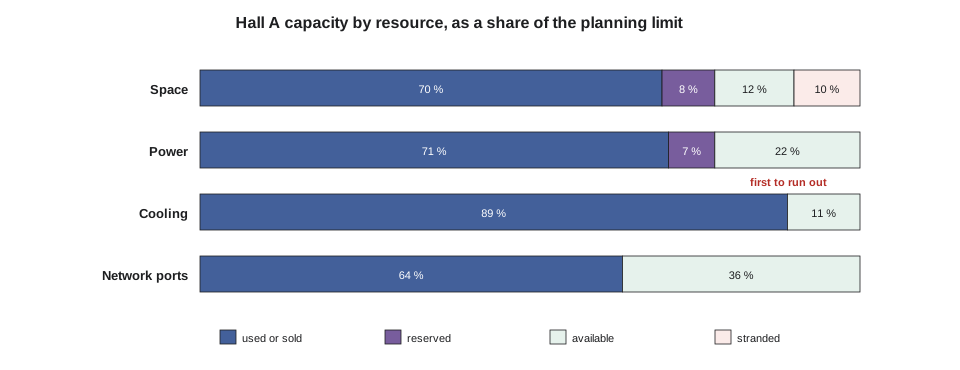
# Hall A capacity dashboard: which resource runs out first?
hall = {  # resource: (planning limit, used, reserved, stranded)
    "space (racks)": (240, 168, 19, 24),
    "power (kW)": (1700, 1205, 120, 0),
    "cooling (kW)": (1350, 1205, 0, 0),
    "network ports": (4800, 3070, 0, 0),
}
first = None
for name, (limit, used, res, strand) in hall.items():
    avail = limit - used - res - strand
    pct = (used + res) / limit * 100
    print(f"{name:14s}: used+reserved {pct:5.1f} %, available {avail:6.0f}, stranded {strand}")
    if first is None or avail / limit < first[1]:
        first = (name, avail / limit)
print(f"First to run out: {first[0]} ({first[1] * 100:.0f} % left)")

space (racks) : used+reserved  77.9 %, available     29, stranded 24
power (kW)    : used+reserved  77.9 %, available    375, stranded 0
cooling (kW)  : used+reserved  89.3 %, available    145, stranded 0
network ports : used+reserved  64.0 %, available   1730, stranded 0
First to run out: cooling (kW) (11 % left)

In Hall A, cooling is the limit: 1,205 kW of measured load against 1,350 kW of usable cooling leaves only 11 %. Selling more power in Hall A would strand it, because there would not be enough cooling to remove the heat. The planners' response was to add rear-door heat exchangers for the next dense customer (DCT-230 lesson 8), raising local cooling capacity without new CRAHs.

Forecasting and early warnings

Capacity changes slowly and then suddenly. A rack's measured load may grow a few percent a month as a customer adds servers, then jump when they install a new generation of hardware. The desk and the planners watch trends: each month's peak load per rack, per row and per hall, against the planning limit. A simple linear trend gives a first estimate of when a limit will be reached; it is not a prediction, but it tells planners which rows to look at.

# Monthly peak load on Hall A row 31 and a simple linear forecast
months = list(range(1, 13))
peaks = [182, 185, 189, 190, 196, 199, 205, 207, 212, 217, 219, 224]   # kW
limit = 260                                                           # row planning limit, kW
n = len(months)
mx, my = sum(months) / n, sum(peaks) / n
slope = sum((x - mx) * (y - my) for x, y in zip(months, peaks)) / sum((x - mx) ** 2 for x in months)
print(f"Growth: about {slope:.1f} kW per month")
left = limit - peaks[-1]
print(f"Headroom now: {left} kW; at this rate the row reaches its limit in about {left / slope:.0f} months")

Growth: about 3.9 kW per month
Headroom now: 36 kW; at this rate the row reaches its limit in about 9 months

Technicians contribute in two ways. They notice the physical signs of growth before the numbers show it: new equipment arriving at the dock for a customer, cages filling up, more tap-off boxes requested. And they record installs and removals in DCIM promptly, because a forecast built on stale records is wrong from the start.