
CON-300 · Lesson 11 of 12 · 28 min
Bid strategy and risk pricing
Two contractors can price the same project with the same cost estimate and still submit very different bids, because the final markup is a strategic decision. Bid too high and the firm loses; bid too low and it wins work that earns nothing or loses money. This lesson looks at the decision from several angles: the winner's curse, simple probabilistic bidding models that use the firm's bid history, the explicit pricing of identified risks, the number of competitors, and unit price strategies such as unbalancing, including where they cross from clever into improper. The models are aids to judgment, not substitutes for it.
The winner's curse
Every estimate contains errors. Some items are overestimated and some underestimated, and on a given project a firm's total estimate may be a few percent high or low compared with what the work will actually cost. When several contractors bid, the one whose estimate is most underestimated is the most likely to be low. Winning therefore tends to select the bids with the largest underestimates, a phenomenon called the winner's curse. The more bidders there are, and the larger the estimating uncertainty, the stronger the effect.
The practical lesson is that a firm's expected profit on the jobs it wins is lower than the markup it adds, on average, unless its estimates are unusually accurate. Firms counter the winner's curse by improving estimate accuracy (better takeoff, leveling and review), bidding fewer projects with more care, investigating large gaps between their bid and the next one (Lesson 10), and adding somewhat more markup when the field is large and uncertainty is high.
import random, statistics
random.seed(7)
# True cost 10.0 ($M); each bidder's estimate has a random error (SD 4 %); all add 5 % markup
true_cost, sd, markup = 10.0, 0.04, 0.05
for n in (2, 4, 8, 12):
    profits = []
    for _ in range(20_000):
        bids = [true_cost * random.gauss(1, sd) * (1 + markup) for _ in range(n)]
        profits.append((min(bids) - true_cost) / true_cost)
    print(f"{n:2d} bidders: average realized margin on cost of the winner "
f"{statistics.mean(profits):+.1%}")2 bidders: average realized margin on cost of the winner +2.6% 4 bidders: average realized margin on cost of the winner +0.7% 8 bidders: average realized margin on cost of the winner -1.0% 12 bidders: average realized margin on cost of the winner -1.8%
In this simulation every bidder intends a 5 % markup, but the winner's realized profit shrinks as the number of bidders grows, and with many bidders the average winner loses money. Real bidders differ in efficiency and markup as well as in estimating error, but the pattern is robust and matches the experience of many contractors in crowded markets.
Probabilistic bidding models
If a contractor keeps a history of its own cost estimates and its competitors' bids, it can estimate the probability that a bid at a given markup would have been lower than each competitor's. A classic approach, associated with Lawrence Friedman's work in the 1950s, records for each past bid the ratio of a competitor's bid to the firm's own estimated cost. The distribution of these ratios shows how often the competitor bid above any given markup. The probability of beating that competitor at markup m is the share of past ratios greater than 1 + m. Assuming competitors bid independently, the probability of beating all of them is the product of the individual probabilities.
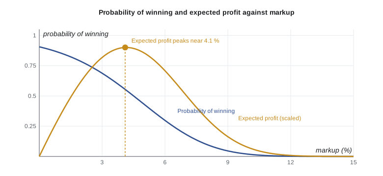
Expected profit is the markup times the cost times the probability of winning. At a low markup the firm wins often but earns little; at a high markup it earns a lot when it wins but rarely wins. The markup that maximizes expected profit lies in between. Other models, such as one proposed by Marvin Gates, combine the competitors' probabilities differently, and modern approaches use regression or machine learning on larger datasets, but the logic is the same.
import random
random.seed(11)
# Bid history: ratios of three known competitors' bids to Northline's estimated cost
history = {
    "Competitor A": [random.gauss(1.075, 0.045) for _ in range(30)],
    "Competitor B": [random.gauss(1.090, 0.055) for _ in range(25)],
    "Competitor C": [random.gauss(1.060, 0.040) for _ in range(18)],
}
cost = 12_000_000
best = None
for pct in range(0, 16, 1):
    m = pct / 100
    p = 1.0
    for ratios in history.values():
        p *= sum(r > 1 + m for r in ratios) / len(ratios)
    ev = m * cost * p
    if best is None or ev > best[2]:
        best = (m, p, ev)
    if pct % 2 == 0:
        print(f"markup {pct:2d} %: P(win) {p:5.2f}  expected profit ${ev:>9,.0f}")
print(f"Best markup about {best[0]:.0%} (P(win) {best[1]:.2f}, expected profit ${best[2]:,.0f})")markup 0 %: P(win) 0.97 expected profit $ 0 markup 2 %: P(win) 0.72 expected profit $ 172,871 markup 4 %: P(win) 0.54 expected profit $ 257,600 markup 6 %: P(win) 0.34 expected profit $ 241,920 markup 8 %: P(win) 0.12 expected profit $ 119,467 markup 10 %: P(win) 0.01 expected profit $ 16,000 markup 12 %: P(win) 0.00 expected profit $ 3,413 markup 14 %: P(win) 0.00 expected profit $ 0 Best markup about 4% (P(win) 0.54, expected profit $257,600)
The model suggests a markup around the point where expected profit peaks. It ignores many things: whether the competitors will actually bid this project, their current workload, the firm's own need for work, the risk profile of this particular project and the strategic value of winning. It also relies on reasonably large, comparable histories, which few firms have for every competitor. Its value is in disciplining the conversation: a firm that habitually bids at a markup with a very low probability of winning, or one that wins almost everything at thin margins, can see it in the numbers.
Worked problem
Expected profit at two markups
For a $9.0 million cost estimate, Northline estimates a 45 % probability of winning at a 4 % markup and a 25 % probability at a 7 % markup. Which markup has the higher expected profit?
Show solution
- At 4 %: profit if won = 0.04 × 9.0 = $360,000; expected = 0.45 × 360,000 = $162,000.
- At 7 %: profit if won = 0.07 × 9.0 = $630,000; expected = 0.25 × 630,000 = $157,500.
Answer: The two are nearly equal. The decision should then turn on factors the model does not capture: how much Northline needs the work, the project risk and the value of the relationship.
Pricing identified risks
Markup is not the only place where risk belongs. Many risks can be identified during the bid and priced explicitly: an aggressive schedule with liquidated damages, a soils report that hints at rock or groundwater, a design that is visibly incomplete in one area, an owner with a history of slow payment, a key subcontractor with limited capacity. A risk register lists each risk with an estimated probability and cost impact. The expected value of each risk (probability times impact) gives a starting point for a risk allowance, and the register shows management where the bid is exposed. CON-350 covers risk management, insurance and bonding in depth; here the focus is on how risk enters the price.
| Risk | Probability | Impact ($) | Expected value ($) | Response |
|---|---|---|---|---|
| Rock in excavation beyond the unit-price allowance | 30 % | 180,000 | 54,000 | Price; clarify unit price in bid |
| Two weeks of liquidated damages from tight schedule | 25 % | 140,000 | 35,000 | Price; plan overtime |
| Curtain wall subcontractor delay | 20 % | 220,000 | 44,000 | Carry second bidder; price partly |
| Owner design changes absorbed under contract terms | 40 % | 60,000 | 24,000 | Price |
| Winter extends beyond plan | 35 % | 75,000 | 26,250 | Price winter weeks |
| Total | 183,250 |
Expected values are a starting point, not a final answer. A firm with limited financial capacity may price large, low-probability risks more heavily because one occurrence could be ruinous. A risk that can be transferred (to a subcontractor through its quote, to an insurer through a policy) or reduced (by a different method or schedule) may need little or no allowance. Risks that remain are either priced explicitly, covered by contingency (Lesson 9) or reflected in the markup. The key is to avoid both double counting (pricing the same risk in contingency and markup) and silent omission.
Competition and the number of bidders
Bid results from public tenders consistently show that the low bid falls, relative to the owner's estimate, as the number of bidders rises. With two or three bidders the low bid is often close to or above the estimate; with eight or ten it is often well below. Contractors use this when deciding both whether to bid (Lesson 1) and how much markup to carry. Information about who obtained documents, who attended the site meeting and which competitors are currently busy or hungry all feeds into the final markup decision. Collusion is illegal (Lesson 1), but intelligence gathered lawfully about the market is part of good bidding.
Unit prices and unbalanced bids
On unit price contracts, the total bid is the sum of each unit price times the owner's estimated quantity, but payment depends on actual quantities. A bidder that believes some quantities are underestimated can raise their unit prices and lower others, keeping the total competitive while increasing revenue if its belief is correct. Raising the prices of items performed early (such as mobilization or excavation) and lowering later items front-loads cash flow. Both are forms of unbalanced bidding.
Owners guard against unbalanced bids. The FAR distinguishes a bid that is mathematically unbalanced (some prices significantly overstated or understated relative to cost) from one that is materially unbalanced (where there is reasonable doubt that award will result in the lowest overall cost to the government, or the bid is so front-loaded it amounts to an advance payment); a materially unbalanced bid may be rejected. State transportation agencies apply similar rules. Front-loading a lump sum contract's schedule of values for cash flow is a related practice; owners and architects reviewing pay applications usually require a schedule of values that reflects the real value of the work.
Worked problem
Detecting an unbalanced bid
The owner's quantities for an earthwork contract are 15,700 yd³ of common excavation and 1,050 yd³ of rock. Bidder X prices common excavation at $10.70 per yd³ and rock at $72.60 per yd³; Bidder Y prices them at $6.90 and $130.00. Compare the totals, then the totals if actual rock is 2,620 yd³ and common excavation 14,130 yd³.
Show solution
- At estimated quantities: X = 15,700 × 10.70 + 1,050 × 72.60 = $244,220; Y = 15,700 × 6.90 + 1,050 × 130 = $244,830.
- At actual quantities: X = 14,130 × 10.70 + 2,620 × 72.60 = $341,403; Y = 14,130 × 6.90 + 2,620 × 130 = $438,097.
Answer: The bids are essentially tied at the owner's quantities, but Bidder Y costs the owner about $96,000 more if rock is underestimated. Bidder Y appears to have unbalanced its prices on the belief that rock is underestimated. An owner that evaluates only at its own quantities would not see the risk.
Estimators should understand unbalancing because they will encounter it from both sides: as bidders deciding how to set unit prices, and as general contractors leveling unit-price quotes from subcontractors. A modest, defensible adjustment based on a genuine view of quantities is common; extreme unbalancing that could not be justified by cost invites rejection, disputes and reputational damage.
Putting the decision together
On bid day, the final markup decision combines several inputs: the firm's target margin for the type of work, the bidding model or bid history, the risk register and contingency, intelligence about competitors, the firm's current backlog and capacity, and the strategic value of the project. Many firms use a short bid review meeting with a standard agenda so that these inputs are discussed every time. Recording the reasoning makes it possible to learn from results: if the firm loses repeatedly by small margins with a particular competitor, or wins and then loses money on a particular type of project, the record shows where the strategy needs to change.
Common mistakes
MistakeAssuming a winning bid will earn the full markup added.
InsteadExpect the winner's curse to reduce realized margins, especially with many bidders and high uncertainty.
MistakeUsing a bidding model as if it decides the markup.
InsteadUse models to discipline judgment, alongside risk, capacity and strategy.
MistakeBurying identified risks in a general markup.
InsteadPrice identified risks explicitly with a risk register; reserve contingency for unidentified variation.
MistakeCounting the same risk in contingency, a risk allowance and markup.
InsteadAssign each risk to one place in the price.
MistakeIgnoring the number of bidders.
InsteadExpect lower low bids with more bidders and adjust go or no-go and markup decisions.
MistakeUnbalancing unit prices to extremes.
InsteadKeep unit prices defensible; materially unbalanced bids can be rejected and cause disputes.
Summary and key terms
- The winner's curse means low bidders tend to be those who underestimated most, especially with many bidders.
- Friedman-style models estimate the probability of beating each competitor from bid history; expected profit is markup times cost times probability of winning.
- The markup that maximizes expected profit lies between low-markup high-probability and high-markup low-probability bids.
- Identified risks should be priced through a risk register using probability and impact, adjusted for the firm's capacity to absorb losses.
- Low bids fall as the number of bidders rises.
- Unbalanced unit prices shift revenue or cash flow; materially unbalanced bids can be rejected.
- A structured bid review combines models, risk, intelligence, capacity and strategy and records the reasoning.
- Winner's curse
- The tendency of the winning bidder to be the one with the largest underestimate.
- Probability of winning
- The estimated chance a bid at a given markup will be lowest.
- Expected profit
- Profit if won multiplied by the probability of winning.
- Friedman model
- A bidding model that multiplies the probabilities of beating each competitor.
- Gates model
- An alternative bidding model combining competitor probabilities differently.
- Risk register
- A list of identified risks with probability, impact and response.
- Expected value of a risk
- Probability times cost impact.
- Unbalanced bid
- A unit price bid with prices that do not reflect cost, shifting revenue or cash flow.
- Materially unbalanced bid
- An unbalanced bid that may not give the owner the lowest overall cost, and may be rejected.
- Front-loading
- Inflating early items to accelerate cash flow.
Practice problems
Work each problem on paper first, then reveal the answer to check.
Explain the winner's curse in one sentence.
Show answer
The lowest bidder is likely to be the one who most underestimated the cost.
Why does the winner's curse grow with more bidders?
Show answer
More bidders make it more likely that one has a large underestimate.
Probabilities of beating three competitors are 0.6, 0.5 and 0.8. Probability of beating all three (independent)?
Show answer
0.24.
Cost $5M, markup 6 %, P(win) 0.3. Expected profit?
Show answer
0.06 × 5,000,000 × 0.3 = $90,000.
Name three things a bidding model ignores.
Show answer
Whether competitors bid, their workload, the firm's need for work, project-specific risk, strategic value.
A risk has a 20 % probability and a $250,000 impact. Expected value?
Show answer
$50,000.
Why might a firm price a large low-probability risk above its expected value?
Show answer
One occurrence could seriously harm a firm with limited financial capacity.
How does the number of bidders tend to affect the low bid?
Show answer
More bidders tend to produce a lower low bid relative to the estimate.
What is front-loading?
Show answer
Raising prices on early items to accelerate cash flow.
When can an unbalanced bid be rejected?
Show answer
When it is materially unbalanced, creating doubt that it gives the owner the lowest overall cost, or under tender terms allowing rejection.
Lesson quiz · 5 questions
Score 60% or more to complete this lesson.
Create a free account to save your progress, take quizzes and earn a certificate.