Logical agents: propositional logic and SAT

A search agent knows only what its problem formulation hard-codes: a list of states and actions. A knowledge-based agent instead keeps a knowledge base of sentences about the world, adds new sentences as it perceives, and derives conclusions by inference. It can be told new facts and goals without being reprogrammed, and it can reach conclusions that were never stated explicitly. This lesson introduces the simplest logic that supports such reasoning, propositional logic, and the algorithms that do the reasoning: model checking, resolution, forward chaining over Horn clauses, and the DPLL and WalkSAT procedures for satisfiability. SAT solving is one of the great success stories of AI and computer science, used daily to verify chips and software.

CMPUT-272 covered the syntax and truth tables of propositional logic and proof by resolution as discrete mathematics. Here the emphasis is on the agent's point of view and on algorithms: how to decide entailment mechanically, how expensive it is, and how modern solvers make an NP-complete problem routinely tractable.

The wumpus world

The wumpus world is a small cave of 4 by 4 squares used to illustrate logical agents. The agent starts in square [1,1]. Somewhere in the cave is a wumpus, a beast that eats anyone entering its square, and some squares contain bottomless pits. One square holds gold. The agent cannot see the hazards directly. Instead, in squares next to (not diagonally) a pit it feels a breeze, in squares next to the wumpus it smells a stench, and in the gold's square it sees a glitter. The agent can move, turn, grab the gold, and shoot its single arrow. The performance measure rewards returning with the gold and heavily penalizes death.

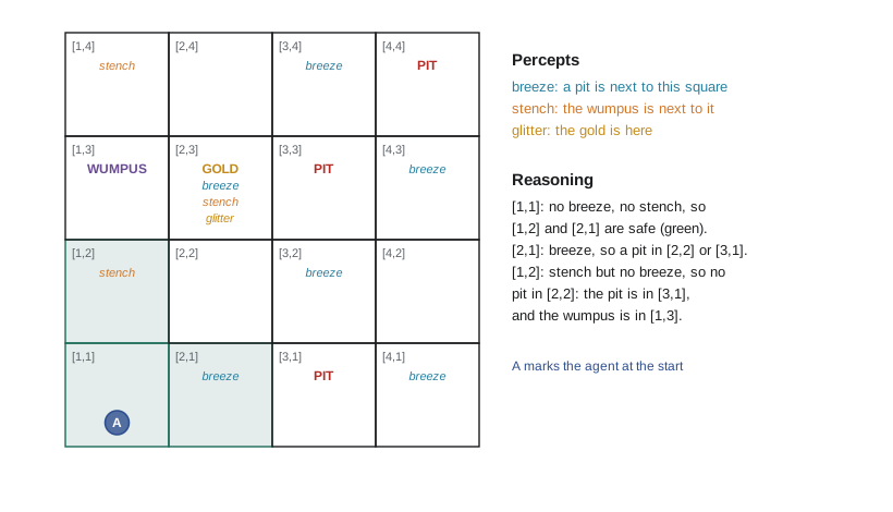
The world is partially observable, so the agent must reason. Starting in [1,1] it perceives no breeze and no stench, so [1,2] and [2,1] are safe. Suppose it moves to [2,1] and feels a breeze. Then a pit is in [2,2] or [3,1] (not [1,1], where it started safely), but it cannot yet say which. Moving back and up to [1,2], it smells a stench but feels no breeze. Now it can conclude that [2,2] has no pit (otherwise [1,2] would be breezy), so the pit is in [3,1]; and the wumpus is not in [2,2] (otherwise [2,1] would have smelled it), so it is in [1,3]. This kind of inference, combining evidence from several percepts, is what a logical agent mechanizes.

Propositional logic

The syntax of propositional logic is simple. Atomic sentences are proposition symbols such as P12 ('there is a pit in [1,2]') or B21 ('there is a breeze in [2,1]'), plus True and False. Complex sentences are built with the connectives ¬ (not), ∧ (and), ∨ (or), ⇒ (implies) and ⇔ (if and only if). The semantics fixes the truth of every sentence relative to a model, an assignment of true or false to every proposition symbol. A ⇒ B is false only when A is true and B is false; A ⇔ B is true when both have the same truth value.

The central notion is entailment. A knowledge base KB entails a sentence α, written KB ⊨ α, if α is true in every model in which KB is true. In other words, there is no way the world could be, consistent with what the agent knows, in which α fails. Entailment is the formal version of 'it follows that'. Two related notions are useful. A sentence is valid if it is true in all models (a tautology, such as P ∨ ¬P), and satisfiable if it is true in at least one. These connect by the deduction theorem: KB ⊨ α if and only if KB ⇒ α is valid, if and only if KB ∧ ¬α is unsatisfiable. That last form is the basis of proof by contradiction, and of most practical reasoning algorithms.

An inference procedure derives sentences from a knowledge base. It is sound if it derives only entailed sentences, and complete if it can derive every entailed sentence. Soundness is essential: an unsound procedure makes things up. Completeness is desirable but sometimes traded away for speed.

Model checking

The most direct way to decide entailment is to enumerate models. Write down every assignment of truth values to the symbols, keep those that satisfy the KB, and check whether the query is true in all of them. With the five rules about the first two squares (no pit in [1,1]; a breeze in a square if and only if a neighboring square has a pit; and the two breeze percepts) and seven symbols, there are 2^7 = 128 models.

# Model checking in the wumpus world: enumerate every model of the relevant symbols.
from itertools import product
SYMBOLS = ["P11", "P12", "P21", "P22", "P31", "B11", "B21"]   # Pxy: pit in square [x,y]; Bxy: breeze felt there

def kb(m):
    return all([
        not m["P11"],                                          # R1: no pit in the start square
        m["B11"] == (m["P12"] or m["P21"]),                    # R2: breeze in [1,1] iff a pit next to it
        m["B21"] == (m["P11"] or m["P22"] or m["P31"]),        # R3: breeze in [2,1] iff a pit next to it
        not m["B11"],                                          # R4: percept: no breeze in [1,1]
        m["B21"],                                              # R5: percept: breeze in [2,1]
    ])

models = [dict(zip(SYMBOLS, vals)) for vals in product([False, True], repeat=len(SYMBOLS))]
kb_models = [m for m in models if kb(m)]
print(f"{len(models)} models enumerated, {len(kb_models)} satisfy the knowledge base")
for query in ["P12", "P21", "P22", "P31"]:
    if all(not m[query] for m in kb_models): verdict = "KB entails no pit: safe"
    elif all(m[query] for m in kb_models):   verdict = "KB entails a pit"
    else:                                     verdict = "unknown: true in some models, false in others"
    print(f"  {query}: {verdict}")

128 models enumerated, 3 satisfy the knowledge base
  P12: KB entails no pit: safe
  P21: KB entails no pit: safe
  P22: unknown: true in some models, false in others
  P31: unknown: true in some models, false in others

Only 3 of the 128 models satisfy the knowledge base. In all of them [1,2] and [2,1] are pit-free, so the KB entails that those squares are safe. [2,2] and [3,1] each have a pit in some models and not in others, so their status is unknown, exactly matching the informal reasoning. Model checking is sound and complete, but it takes time O(2^n) for n symbols; a real wumpus world with 16 squares and several kinds of fact has dozens of symbols, and real verification problems have millions. Deciding entailment in propositional logic is co-NP-complete, so no algorithm is efficient in the worst case, but the algorithms below are far better than enumeration on typical problems.

Inference rules and resolution

Theorem proving derives conclusions by applying inference rules directly to sentences, without enumerating models. The best known rule is modus ponens: from α ⇒ β and α, infer β. And-elimination infers α from α ∧ β. Logical equivalences, such as De Morgan's laws ¬(α ∧ β) ≡ ¬α ∨ ¬β and the elimination of implication α ⇒ β ≡ ¬α ∨ β, let us rewrite sentences. Searching for a proof is itself a search problem, and on many problems a proof is found in far fewer steps than there are models, because irrelevant symbols are simply ignored.

A single rule, resolution, is enough for a complete inference procedure. It works on clauses, disjunctions of literals, where a literal is a symbol or its negation. From the clauses (ℓ1 ∨ … ∨ ℓk ∨ x) and (m1 ∨ … ∨ mn ∨ ¬x), resolution infers the resolvent (ℓ1 ∨ … ∨ ℓk ∨ m1 ∨ … ∨ mn): x is either true or false, so one of the remaining parts must hold. Every sentence can be converted to conjunctive normal form (CNF), a conjunction of clauses, by eliminating ⇔ and ⇒, pushing negations inward with De Morgan's laws, and distributing ∨ over ∧.

To prove KB ⊨ α by resolution, convert KB ∧ ¬α to CNF and resolve pairs of clauses repeatedly. If the empty clause appears, the set is unsatisfiable, so the entailment holds. If no new clauses can be added, it does not. Resolution is sound, and by the ground resolution theorem it is refutation-complete: if the set of clauses is unsatisfiable, resolution will eventually derive the empty clause.

# Resolution refutation: prove KB |= not P12 by deriving the empty clause from KB and P12.
# Clauses are frozensets of literals; "-X" is the negation of X. The KB is already in CNF.
from itertools import combinations
KB = [{"-P11"},
      {"-B11", "P12", "P21"}, {"-P12", "B11"}, {"-P21", "B11"},              # B11 <=> P12 or P21
      {"-B21", "P11", "P22", "P31"}, {"-P11", "B21"}, {"-P22", "B21"}, {"-P31", "B21"},
      {"-B11"}, {"B21"}]
neg = lambda l: l[1:] if l.startswith("-") else "-" + l

def resolve(c1, c2):
    out = []
    for l in c1:
        if neg(l) in c2:
            r = (c1 - {l}) | (c2 - {neg(l)})
            if not any(neg(x) in r for x in r):        # skip tautologies
                out.append(frozenset(r))
    return out

def refute(clauses):
    clauses = set(map(frozenset, clauses)); derived = {}
    while True:
        new = set()
        for c1, c2 in combinations(sorted(clauses, key=sorted), 2):
            for r in resolve(c1, c2):
                if r not in clauses and r not in new: derived[r] = (c1, c2)
                new.add(r)
                if not r: return derived, len(clauses)
        if new <= clauses: return None, len(clauses)
        clauses |= new

def show(c): return "{" + ", ".join(sorted(c)) + "}" if c else "{} (the empty clause)"
derived, n = refute(KB + [{"P12"}])                         # add the negated query: P12
print("empty clause derived, so KB entails not P12; proof:")
def trace(c, depth=0):
    if c in derived:
        a, b = derived[c]; trace(a, depth + 1); trace(b, depth + 1)
        print("  " * depth + show(c) + "   from " + show(a) + " and " + show(b))
trace(frozenset())

empty clause derived, so KB entails not P12; proof:
  {B11}   from {-P12, B11} and {P12}
{} (the empty clause)   from {-B11} and {B11}

The proof is short: assuming a pit in [1,2], the clause ¬P12 ∨ B11 (one direction of the breeze rule) gives a breeze in [1,1], which contradicts the percept ¬B11. The program added the negated query and searched until it derived the empty clause. Plain resolution generates many useless clauses on larger problems; refinements such as the set-of-support strategy (always resolve with a clause descended from the negated query) and unit preference (prefer resolving with single-literal clauses) keep it focused.

Horn clauses, forward and backward chaining

Many knowledge bases need only a restricted form of clause. A definite clause has exactly one positive literal; written as an implication, it is (P1 ∧ … ∧ Pk) ⇒ Q, a rule whose premises are all positive. A fact is a definite clause with no premises. Horn clauses allow at most one positive literal, so they also include goal clauses with none. Entailment with Horn clauses can be decided in time linear in the size of the knowledge base, which is why they underlie Prolog, Datalog and production-rule systems.

Forward chaining starts from the known facts and fires any rule whose premises are all known, adding its conclusion, until the query is derived or nothing new can be added. It keeps, for each rule, a count of premises not yet known, so each rule is examined only when one of its premises becomes known. It is sound and complete for definite clauses, and it is data-driven: it derives everything that follows from the facts, relevant or not.

# Forward chaining over Horn clauses: fire each rule once all its premises are known.
RULES = [  # (premises, conclusion)
    (["StenchFelt12"], "WumpusNear12"),
    (["GlitterSeen22"], "GoldIn22"),
    (["NoBreeze11"], "NoPit12"), (["NoBreeze11"], "NoPit21"),
    (["NoPit12", "NoWumpus12"], "Safe12"),
    (["NoPit21", "NoWumpus21"], "Safe21"),
    (["NoStench11"], "NoWumpus12"), (["NoStench11"], "NoWumpus21"),
    (["Safe12", "Safe21"], "TwoExitsSafe"),
]
FACTS = ["NoBreeze11", "NoStench11"]

def forward_chain(rules, facts, query):
    count = {i: len(p) for i, (p, _) in enumerate(rules)}       # premises still unknown per rule
    known, agenda, fired = set(), list(facts), 0
    while agenda:
        p = agenda.pop(0)
        if p in known: continue
        known.add(p); print("  known:", p)
        if p == query: return True, fired
        for i, (prem, concl) in enumerate(rules):
            if p in prem:
                count[i] -= 1
                if count[i] == 0: agenda.append(concl); fired += 1
    return False, fired

ok, fired = forward_chain(RULES, FACTS, "TwoExitsSafe")
print(f"query proved: {ok}; rules fired: {fired} of {len(RULES)}")

  known: NoBreeze11
  known: NoStench11
  known: NoPit12
  known: NoPit21
  known: NoWumpus12
  known: NoWumpus21
  known: Safe12
  known: Safe21
  known: TwoExitsSafe
query proved: True; rules fired: 7 of 9

Backward chaining works from the query instead. To prove Q, it finds rules concluding Q and tries to prove each of their premises in turn, recursively, until it reaches known facts. It is goal-driven, touching only facts relevant to the query, so it is often much faster than forward chaining for answering specific questions. Prolog is a backward-chaining engine for first-order Horn clauses, as lesson 8 explains, and CMPUT-325 builds one. Forward chaining suits agents that must react to new percepts as they arrive; backward chaining suits agents answering questions.

Satisfiability: DPLL

Because KB ⊨ α exactly when KB ∧ ¬α is unsatisfiable, an efficient satisfiability (SAT) solver gives efficient entailment. SAT was the first problem proved NP-complete (Cook, 1971), yet modern solvers routinely decide formulas with millions of clauses. The foundation is the DPLL algorithm (Davis, Putnam, Logemann and Loveland, 1962). It is a backtracking search over truth assignments, like the CSP backtracking of lesson 6, with three improvements over enumerating models:

The program implements DPLL and runs it on random 3-SAT formulas: each clause has three distinct variables, each negated with probability one half. With n = 50 variables we vary the number of clauses m and record the fraction of satisfiable formulas and the number of recursive calls.

# DPLL with unit propagation and pure literals, tested on random 3-SAT across the phase transition.
import random

def dpll(clauses, assignment, stats):
    stats["calls"] += 1
    while True:                                               # simplify until nothing changes
        clauses = [c for c in clauses if not any(assignment.get(abs(l)) == (l > 0) for l in c)]
        clauses = [[l for l in c if abs(l) not in assignment] for c in clauses]
        if not clauses: return assignment                     # every clause satisfied
        if any(not c for c in clauses): return None           # an empty clause: conflict
        units = [c[0] for c in clauses if len(c) == 1]
        lits = {l for c in clauses for l in c}
        pures = [l for l in lits if -l not in lits]
        if not units and not pures: break
        for l in units + pures: assignment = {**assignment, abs(l): l > 0}
    counts = {}
    for c in clauses:
        for l in c: counts[abs(l)] = counts.get(abs(l), 0) + 1
    var = max(sorted(counts), key=counts.get)                 # branch on the most frequent variable
    for value in (True, False):
        result = dpll(clauses, {**assignment, var: value}, stats)
        if result is not None: return result
    return None

def random_3sat(n, m, rng):
    return [[v if rng.random() < 0.5 else -v for v in rng.sample(range(1, n + 1), 3)] for _ in range(m)]

rng, n = random.Random(366), 50
print(" m/n   satisfiable   mean DPLL calls")
for ratio in (3.0, 3.6, 4.0, 4.3, 4.6, 5.0, 6.0):
    sat = calls = 0
    for _ in range(30):
        f = random_3sat(n, round(ratio * n), rng); stats = {"calls": 0}
        model = dpll(f, {}, stats)
        if model is not None:
            assert all(any(model.get(abs(l), True) == (l > 0) for l in c) for c in f)   # check the model
            sat += 1
        calls += stats["calls"]
    print(f"{ratio:4.1f} {sat / 30:10.0%} {calls / 30:14.1f}")

 m/n   satisfiable   mean DPLL calls
 3.0       100%           12.9
 3.6       100%           31.9
 4.0        90%           66.3
 4.3        77%           76.6
 4.6        20%           90.9
 5.0         3%           89.0
 6.0         0%           54.3

The results show the famous phase transition. With few clauses per variable, almost every formula is satisfiable and DPLL finds a model quickly. With many, almost every formula is unsatisfiable and contradictions appear quickly. Between ratios of about 4 and 5, the probability of satisfiability drops sharply from near 1 to near 0, and that is exactly where the formulas are hardest, with the most recursive calls. For large n the transition sharpens around m/n ≈ 4.27. The lesson generalizes beyond SAT: the hardest instances of many constraint problems sit at the boundary between under-constrained and over-constrained, a phenomenon we also met with min-conflicts in lesson 6.

Modern solvers extend DPLL into conflict-driven clause learning (CDCL). When a branch fails, the solver analyzes the chain of unit propagations that led to the conflict and learns a new clause that rules out its cause, the nogood learning of lesson 6, and then backjumps non-chronologically to the level where that clause becomes useful. Add clever data structures (two watched literals per clause make unit propagation fast), variable selection that favors variables involved in recent conflicts, and frequent restarts, and the result is the solvers, such as MiniSat and CaDiCaL, that verify microprocessor designs, check software and solve planning problems by encoding them in logic (lesson 11).

Satisfiability: local search

Local search also applies to SAT. WalkSAT starts from a random assignment and repeatedly picks an unsatisfied clause. With probability p it flips a random variable from that clause (a random-walk move); otherwise it flips the variable in the clause that leaves the fewest clauses unsatisfied (a greedy move, like min-conflicts). If it finds a model, the formula is satisfiable; but if it fails within its flip limit, we learn nothing, since it cannot prove unsatisfiability. WalkSAT is therefore useful when we expect a solution to exist, as in planning and scheduling, and useless for proving entailment, which requires showing that KB ∧ ¬α has no model.

# WalkSAT on satisfiable random 3-SAT formulas (seeded): local search with random-walk moves.
import random

def walksat(clauses, n, rng, p=0.5, max_flips=100000):
    model = {v: rng.random() < 0.5 for v in range(1, n + 1)}
    sat = lambda c: any(model[abs(l)] == (l > 0) for l in c)
    for flips in range(max_flips):
        unsat = [c for c in clauses if not sat(c)]
        if not unsat: return model, flips
        c = rng.choice(unsat)
        if rng.random() < p:
            v = abs(rng.choice(c))                             # random walk move
        else:                                                  # greedy move: flip the best variable
            def broken_after(v):
                model[v] = not model[v]; k = sum(not sat(d) for d in clauses); model[v] = not model[v]
                return k
            v = min(sorted(abs(l) for l in c), key=broken_after)
        model[v] = not model[v]
    return None, max_flips

rng = random.Random(366)
for n in (50, 100, 200):
    hidden = {v: rng.random() < 0.5 for v in range(1, n + 1)}      # plant a solution so one exists
    clauses = []
    while len(clauses) < int(4.0 * n):
        c = [v if rng.random() < 0.5 else -v for v in rng.sample(range(1, n + 1), 3)]
        if any(hidden[abs(l)] == (l > 0) for l in c): clauses.append(c)
    model, flips = walksat(clauses, n, rng)
    print(f"n = {n:3}, {len(clauses)} clauses: {'solved' if model else 'not solved'} after {flips:,} flips")

n =  50, 200 clauses: solved after 343 flips
n = 100, 400 clauses: solved after 451 flips
n = 200, 800 clauses: solved after 586 flips

Building a logical agent

A wumpus agent built on propositional logic would keep a knowledge base containing the rules of the world (for every square, B[x,y] ⇔ a pit in some adjacent square, and similarly for stenches), add its percepts as they arrive, and before each move ask whether each candidate square is provably safe. It would move to a provably safe unvisited square if one exists, and otherwise take the least risky move, which requires probability (lesson 9). Two difficulties appear quickly. First, the rules must be written separately for every square, because propositional logic has no variables; a 4 by 4 cave needs dozens of near-identical sentences, and the clauses multiply when time matters, because facts such as 'the agent is in [1,1]' change, so each needs a time index (L11 at time 0, L12 at time 1) and successor-state axioms that say how actions change them. Second, the agent can be certain only of what follows logically; it cannot weigh likelihoods. Lesson 8 addresses the first difficulty with first-order logic, and lesson 9 the second with probability.

Worked examples