Classical planning

A search agent in lesson 3 needed a hand-crafted heuristic for every new problem, and its states were opaque. A planning agent represents states and actions in a factored, logical language, so a single general-purpose planner can solve problems in any domain described in that language, and can compute its own heuristics from the description. This lesson introduces classical planning: the STRIPS representation and its modern standard, PDDL; forward and backward state-space search; domain-independent heuristics derived by relaxing the problem; planning graphs and GraphPlan; and the alternatives of partial-order, hierarchical and SAT-based planning. It ends with how planning is used in practice and how it connects to the other methods of this course.

Classical planning assumes a world that is fully observable, deterministic, static and discrete, with a single agent: the easy end of every dimension in lesson 1's table. That sounds restrictive, but many real problems are close enough, and the techniques extend. The Shakey robot project at SRI (1966–1972) produced both STRIPS and A*; NASA's Remote Agent planned and executed actions on board the Deep Space 1 spacecraft in 1999; and planners schedule observations, logistics, manufacturing and game characters today. ROB-340 studies motion planning in continuous spaces; here the focus is task planning, deciding what to do and in what order.

Representing planning problems

In the STRIPS representation (Fikes and Nilsson, 1971), a state is a set of ground atoms, facts that are true, such as at(robot, mailroom) and at(p1, mailroom); every atom not listed is false (the closed-world assumption). An action schema has a name with parameters, a precondition (a set of atoms that must hold for the action to apply), and an effect, given as an add list of atoms that become true and a delete list of atoms that become false. The result of applying action a in state s is (s − Del(a)) ∪ Add(a). A goal is a set of atoms that must all hold; any state containing them is a goal state.

The key idea is that atoms not mentioned in an action's effects keep their values. This solves the frame problem, the difficulty of saying what does not change, which in first-order logic needs many explicit frame axioms. STRIPS buys this convenience by restricting what can be said: no conditional effects, no disjunctive goals, no numbers. The Planning Domain Definition Language (PDDL), introduced for the first International Planning Competition in 1998, is the standard successor. It keeps STRIPS at its core and adds optional features such as types, negative preconditions, conditional effects, numeric fluents, durative actions and preferences. A PDDL task is split into a domain file, with the predicates and action schemas, and a problem file, with the objects, initial state and goal.

; domain file
(define (domain delivery)
  (:requirements :strips :typing)
  (:types room parcel)
  (:predicates (robot-at ?r - room) (at ?p - parcel ?r - room)
               (holding ?p - parcel) (door ?a ?b - room))
  (:action move
    :parameters (?a ?b - room)
    :precondition (and (robot-at ?a) (door ?a ?b))
    :effect (and (robot-at ?b) (not (robot-at ?a))))
  (:action pick
    :parameters (?p - parcel ?r - room)
    :precondition (and (robot-at ?r) (at ?p ?r))
    :effect (and (holding ?p) (not (at ?p ?r))))
  (:action drop
    :parameters (?p - parcel ?r - room)
    :precondition (and (robot-at ?r) (holding ?p))
    :effect (and (at ?p ?r) (not (holding ?p)))))

; problem file
(define (problem three-parcels)
  (:domain delivery)
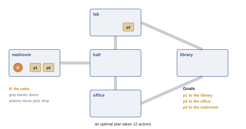
  (:objects mailroom hall lab office library - room  p1 p2 p3 - parcel)
  (:init (robot-at mailroom) (at p1 mailroom) (at p2 mailroom) (at p3 lab)
         (door mailroom hall) (door hall mailroom) (door hall lab) (door lab hall)
         (door hall office) (door office hall) (door office library)
         (door library office) (door lab library) (door library lab))
  (:goal (and (at p1 library) (at p2 office) (at p3 mailroom))))

The delivery domain

Our running example is a robot that delivers parcels between five rooms of a campus building. It can move through a door between adjacent rooms, pick up a parcel in its room, and drop a parcel it is holding. Parcels p1 and p2 start in the mailroom and must go to the library and the office; parcel p3 starts in the lab and must go back to the mailroom. Grounding the three schemas over all rooms and parcels gives 40 concrete actions. The program below encodes the problem in STRIPS style and solves it by forward search with several heuristics.

Forward state-space search

Forward search, or progression, starts at the initial state and applies applicable actions to reach new states, exactly like the search algorithms of lessons 2 and 3. Its difficulty is the branching factor. Real domains have many irrelevant actions: a robot in a building with 100 rooms and 1,000 parcels can move in several directions and could pick up any parcel in its room, and most of these choices are pointless. Uninformed forward search drowns in them. For decades this made forward search look hopeless for planning, until the late 1990s, when planners such as HSP and FF showed that domain-independent heuristics computed automatically from the action descriptions make forward search the most effective approach.

# A STRIPS planning problem: a campus delivery robot moves parcels between rooms.
from itertools import product
ROOMS = ["mailroom", "hall", "lab", "office", "library"]
DOORS = [("mailroom", "hall"), ("hall", "lab"), ("hall", "office"), ("office", "library"), ("lab", "library")]
PARCELS = ["p1", "p2", "p3"]

def ground_actions():
    acts = []      # each action: (name, preconditions, add list, delete list)
    links = DOORS + [(b, a) for a, b in DOORS]
    for a, b in links:
        acts.append((f"move({a},{b})", {f"at(robot,{a})"}, {f"at(robot,{b})"}, {f"at(robot,{a})"}))
    for p, r in product(PARCELS, ROOMS):
        acts.append((f"pick({p},{r})", {f"at(robot,{r})", f"at({p},{r})"}, {f"holding({p})"}, {f"at({p},{r})"}))
        acts.append((f"drop({p},{r})", {f"at(robot,{r})", f"holding({p})"}, {f"at({p},{r})"}, {f"holding({p})"}))
    return acts

ACTIONS = ground_actions()
INIT = frozenset({"at(robot,mailroom)", "at(p1,mailroom)", "at(p2,mailroom)", "at(p3,lab)"})
GOAL = {"at(p1,library)", "at(p2,office)", "at(p3,mailroom)"}

def applicable(state):
    return [a for a in ACTIONS if a[1] <= state]
def result(state, a):
    return frozenset((state - a[3]) | a[2])

import heapq
from collections import deque

def bfs():
    frontier, seen, expanded = deque([(INIT, [])]), {INIT}, 0
    while frontier:
        s, plan = frontier.popleft()
        if GOAL <= s: return plan, expanded
        expanded += 1
        for a in applicable(s):
            t = result(s, a)
            if t not in seen: seen.add(t); frontier.append((t, plan + [a[0]]))

def relaxed_costs(state, combine):
    """Cost of reaching each fact when delete lists are ignored; combine is sum (h_add) or max (h_max)."""
    cost = {f: 0 for f in state}
    changed = True
    while changed:
        changed = False
        for name, pre, add, _ in ACTIONS:
            if all(p in cost for p in pre):
                c = 1 + combine([cost[p] for p in pre])
                for f in add:
                    if c < cost.get(f, 1e9): cost[f] = c; changed = True
    return combine([cost.get(g, 1e9) for g in GOAL])

def h_add(state): return relaxed_costs(state, sum)
def h_max(state): return relaxed_costs(state, max)

def goal_count(state): return sum(g not in state for g in GOAL)

def best_first(h, weight=1.0):
    frontier, g, expanded, tie = [(weight * h(INIT), 0, 0, INIT, [])], {INIT: 0}, 0, 1
    while frontier:
        _, gs, _, s, plan = heapq.heappop(frontier)
        if GOAL <= s: return plan, expanded
        if gs > g[s]: continue
        expanded += 1
        for a in applicable(s):
            t = result(s, a)
            if gs + 1 < g.get(t, 1e9):
                g[t] = gs + 1; tie += 1
                heapq.heappush(frontier, (gs + 1 + weight * h(t), gs + 1, tie, t, plan + [a[0]]))

print(len(ACTIONS), "ground actions")
plan, n = bfs()
print(f"breadth-first:                        plan length {len(plan):2}, states expanded {n:5}")
plan2, n2 = best_first(goal_count)
print(f"A* with goal count:                   plan length {len(plan2):2}, states expanded {n2:5}")
plan4, n4 = best_first(h_max)
print(f"A* with h_max (admissible):           plan length {len(plan4):2}, states expanded {n4:5}")
plan3, n3 = best_first(h_add)
print(f"A* order with h_add (not admissible): plan length {len(plan3):2}, states expanded {n3:5}")
print("plan:", ", ".join(plan))

40 ground actions
breadth-first:                        plan length 12, states expanded  1003
A* with goal count:                   plan length 12, states expanded   644
A* with h_max (admissible):           plan length 12, states expanded   446
A* order with h_add (not admissible): plan length 12, states expanded    21
plan: pick(p1,mailroom), pick(p2,mailroom), move(mailroom,hall), move(hall,lab), pick(p3,lab), move(lab,library), drop(p1,library), move(library,office), drop(p2,office), move(office,hall), move(hall,mailroom), drop(p3,mailroom)

Breadth-first search finds a 12-step plan after expanding about a thousand states. A* with the goal-count heuristic (the number of unsatisfied goal atoms) expands about 640; with h_max it expands about 450; and ordering the search by h_add expands only 21 states, still finding a 12-step plan, although h_add does not guarantee optimality. The heuristics knew nothing about robots or parcels: they were computed from the action schemas alone. On larger problems the gap grows exponentially, which is why every competitive planner relies on such heuristics.

Heuristics from relaxed problems

Lesson 3 showed that the exact cost of a relaxed problem is an admissible heuristic. Planning heuristics come from relaxations that the factored representation makes easy to compute. Ignoring preconditions makes every action applicable everywhere, so the heuristic counts roughly how many actions are needed to achieve the goals; goal counting is a crude version of this, admissible here because each action achieves at most one goal atom but not in general. Ignoring delete lists is more informative: in the delete relaxation, facts once achieved stay true forever, so the relaxed problem has no conflicts between goals and progress is monotonic.

Finding an optimal relaxed plan is still NP-hard, so planners estimate it. h_max sets the cost of a set of facts to the cost of the most expensive one; it is admissible but often weak. h_add sums the costs of the facts; it is much more informative but can overcount when actions achieve several facts at once, so it is not admissible. The FF heuristic extracts an actual relaxed plan and counts its actions, giving estimates between the two. Landmarks, facts that every plan must achieve at some point (in our problem, holding(p3) and at(robot, lab)), provide another powerful source of heuristic information and are used in the LAMA planner, which won the 2008 planning competition.

Backward search

Backward search, or regression, starts from the goal and works toward the initial state. Instead of states it searches over descriptions: sets of atoms that must hold. An action a is relevant to a goal description g if it achieves some atom of g and deletes none; regressing g through a gives g′ = (g − Add(a)) ∪ Pre(a), the description of states from which doing a reaches g. Backward search considers only relevant actions, so its branching factor is often much smaller than that of forward search. However, its descriptions are partial states, which makes good heuristics harder to compute, and in practice forward search with strong heuristics has been more successful.

Planning graphs and GraphPlan

A planning graph is a layered structure that over-approximates which facts could be true after each number of steps. Level 0 holds the initial facts. Each action level contains every action whose preconditions appear in the previous fact level, plus no-op actions that carry facts forward; the next fact level holds every fact added by those actions. GraphPlan (Blum and Furst, 1995) also records mutual exclusion (mutex) relations: two actions are mutex if one deletes a precondition or effect of the other, or if their preconditions are mutex; two facts are mutex if every way of achieving them both involves mutex actions. The graph grows only polynomially, leveling off once no new facts or mutexes appear.

# A STRIPS planning problem: a campus delivery robot moves parcels between rooms.
from itertools import product
ROOMS = ["mailroom", "hall", "lab", "office", "library"]
DOORS = [("mailroom", "hall"), ("hall", "lab"), ("hall", "office"), ("office", "library"), ("lab", "library")]
PARCELS = ["p1", "p2", "p3"]

def ground_actions():
    acts = []      # each action: (name, preconditions, add list, delete list)
    links = DOORS + [(b, a) for a, b in DOORS]
    for a, b in links:
        acts.append((f"move({a},{b})", {f"at(robot,{a})"}, {f"at(robot,{b})"}, {f"at(robot,{a})"}))
    for p, r in product(PARCELS, ROOMS):
        acts.append((f"pick({p},{r})", {f"at(robot,{r})", f"at({p},{r})"}, {f"holding({p})"}, {f"at({p},{r})"}))
        acts.append((f"drop({p},{r})", {f"at(robot,{r})", f"holding({p})"}, {f"at({p},{r})"}, {f"holding({p})"}))
    return acts

ACTIONS = ground_actions()
INIT = frozenset({"at(robot,mailroom)", "at(p1,mailroom)", "at(p2,mailroom)", "at(p3,lab)"})
GOAL = {"at(p1,library)", "at(p2,office)", "at(p3,mailroom)"}

def applicable(state):
    return [a for a in ACTIONS if a[1] <= state]
def result(state, a):
    return frozenset((state - a[3]) | a[2])

# A relaxed planning graph: the level at which each fact first appears when delete lists are ignored.
level, facts, k = {f: 0 for f in INIT}, set(INIT), 0
while not GOAL <= facts:
    k += 1
    new = set()
    for name, pre, add, _ in ACTIONS:
        if pre <= facts: new |= add - facts
    if not new: break
    for f in new: level[f] = k
    facts |= new
for f in sorted(level, key=lambda f: (level[f], f)):
    if f.startswith("at(p") or f.startswith("holding"): print(f"level {level[f]}: {f}")
print("h_max (deepest goal level) =", max(level[g] for g in GOAL), "; h_level sum =", sum(level[g] for g in GOAL))

level 0: at(p1,mailroom)
level 0: at(p2,mailroom)
level 0: at(p3,lab)
level 1: holding(p1)
level 1: holding(p2)
level 2: at(p1,hall)
level 2: at(p2,hall)
level 3: at(p1,lab)
level 3: at(p1,office)
level 3: at(p2,lab)
level 3: at(p2,office)
level 3: holding(p3)
level 4: at(p1,library)
level 4: at(p2,library)
level 4: at(p3,hall)
level 4: at(p3,library)
level 4: at(p3,mailroom)
level 4: at(p3,office)
h_max (deepest goal level) = 4 ; h_level sum = 11

The level at which a fact first appears is an admissible estimate of the number of steps needed to achieve it, and the maximum level over the goals, 4 here, is the h_max heuristic counted in steps. The true optimal plan needs 12 steps because the robot can be in only one place at a time; the relaxed graph, which ignores deletes and therefore mutexes, lets it be everywhere at once. GraphPlan uses the full graph with mutexes to find plans directly: once all goals appear in a fact level with no pair of them mutex, it searches backward through the graph for a set of non-mutex actions at each level that achieves them, extending the graph and trying again if the search fails. GraphPlan was a breakthrough in the late 1990s; today its main legacy is the planning-graph heuristics used by forward-search planners.

Planning as satisfiability

Another approach compiles planning into the SAT problems of lesson 7. Choose a horizon T. Create propositional variables for every fact at every time step 0 to T and for every action at every step 0 to T − 1. Add clauses for the initial state at time 0 and the goal at time T, clauses saying that an action at step t implies its preconditions at t and its effects at t + 1, frame axioms saying that facts change only when some action changes them, and exclusion axioms preventing incompatible actions at the same step. Any model of the formula is a plan. If the formula is unsatisfiable, increase T and try again. Kautz and Selman's SATPLAN showed in the 1990s that this can beat specialized planners, and modern SAT solvers keep the approach competitive, particularly for problems where proving that no shorter plan exists matters.

Partial-order and hierarchical planning

State-space planners produce totally ordered plans, a single sequence of steps. Partial-order planners instead search the space of partial plans, adding steps, causal links (step A achieves precondition p of step B) and ordering constraints, and resolving threats, steps that might delete p between A and B. The result commits only to the orderings that matter, which is useful when a plan will be executed by several agents in parallel or must be adjusted on the fly: in our domain, picking up p1 and p2 can happen in either order. Partial-order planning dominated the field in the 1980s and early 1990s and remains useful for plan explanation and multi-agent execution.

Hierarchical task network (HTN) planning works more like a human planner, refining high-level tasks into lower-level ones. A method for the task deliver(p, r) might decompose it into go to p's room, pick up p, go to r and drop p, and go to(r) might decompose into a sequence of moves. The planner searches over decompositions rather than individual actions, guided by methods that encode expert knowledge of how tasks are usually done. HTN planners such as SHOP2 have been used in manufacturing, evacuation planning and game AI, and hierarchical structure is how most practical planning systems scale.

Planning in the real world

Real problems break the classical assumptions. Time and resources need durative actions and numeric fluents, which PDDL 2.1 added, as in scheduling a planetary rover's instruments around battery charge and communication windows. Uncertainty about action outcomes leads to MDPs (lesson 10) and to contingent plans with sensing actions; incomplete knowledge of the initial state leads to conformant planning, plans that work whatever the true state. And because the world changes during execution, a deployed agent must monitor execution and replan when something goes wrong, which most robot architectures do continuously, as lesson 12's capstone agent will. NASA's Mars rovers, warehouse robot fleets and video-game characters all combine a planner with this kind of execution monitoring.

Planning also connects to the rest of the course. Forward planning is heuristic search (lesson 3) with automatically derived heuristics. Scheduling with resource constraints is constraint satisfaction (lesson 6). Planning as SAT is logical inference (lesson 7), and planning in first-order domains uses unification (lesson 8). Planning under uncertainty uses probabilistic models and decision theory (lessons 9 and 10). Recent research also asks whether large language models can plan. On standard PDDL benchmarks they have generally been less reliable than classical planners, especially as problems grow, so a common design pairs them: the language model translates a request into PDDL, and a planner or plan verifier guarantees that the resulting plan is correct.

Worked examples