Making decisions: utility, value of information and MDPs

Lesson 9 gave the agent beliefs; this lesson tells it what to do with them. A rational agent under uncertainty should choose the action with the highest expected utility: weigh each possible outcome by how likely it is and how much the agent wants it. That principle, simple to state, has deep foundations and wide consequences. This lesson develops utility theory, applies it to single decisions, computes the value of gathering information before deciding, and then extends it to sequential decisions in Markov decision processes (MDPs), solved by value iteration and policy iteration on a gridworld.

Decision theory is shared ground between AI, economics, statistics and operations research. AI-330 takes MDPs much further, into reinforcement learning, where the agent does not know the transition model or rewards and must learn from experience; that field was shaped by Richard Sutton and Andrew Barto, whose work is closely associated with the University of Alberta and the Alberta Machine Intelligence Institute (Amii). Here we assume the model is known and focus on computing good decisions.

Expected utility

An agent's preferences over outcomes are captured by a utility function U(s), which assigns a number to each state. If an action a can lead to outcomes s′ with probabilities P(s′ | a, e) given evidence e, its expected utility is

and the principle of maximum expected utility (MEU) says a rational agent chooses the action that maximizes it. Expectimax in lesson 5 was MEU applied to game trees. The principle tells the agent how to act given its beliefs and preferences; it does not say where those come from. Beliefs come from probabilistic reasoning, and preferences from the designer, the user, or learning.

Why utilities exist

Why should preferences be represented by numbers at all, and why should the agent maximize their expectation rather than, say, avoid the worst case? Von Neumann and Morgenstern answered in 1944. Consider lotteries, situations with uncertain prizes, written [p, A; 1 − p, B]. Suppose an agent's preferences among lotteries obey six axioms: orderability (any two lotteries are comparable), transitivity (if A ≻ B and B ≻ C then A ≻ C), continuity, substitutability, monotonicity and decomposability. Then there exists a utility function U such that the agent prefers lottery L1 to L2 exactly when the expected utility of L1 is higher. Violating the axioms has consequences: an agent with intransitive preferences (A ≻ B, B ≻ C, C ≻ A) can be led around a cycle of trades, paying a small fee each time, as a money pump.

Utility functions are unique only up to positive linear transformations: U′(s) = aU(s) + b with a > 0 describes the same preferences, which is why the scale of an evaluation function mattered for expectimax but not for minimax. A common normalization sets the best possible prize to 1 and the worst to 0, and assesses the utility of any intermediate outcome S as the probability p at which the agent is indifferent between S for sure and the standard lottery [p, best; 1 − p, worst].

The utility of money and attitudes to risk

Money is the most familiar example where utility differs from face value. Most people would refuse an even bet to double or halve their savings, even though its expected monetary value (EMV) is positive. Their utility for money is concave: each extra dollar is worth a little less than the one before. An agent with a concave utility is risk-averse, preferring a sure amount to a gamble with the same EMV; one with a linear utility is risk-neutral; one with a convex utility is risk-seeking. The certainty equivalent of a lottery is the sure amount the agent values equally, and the gap between the EMV and the certainty equivalent is the risk premium.

# Expected utility with a concave utility for money: risk aversion and insurance.
import math
wealth = 40000
lottery = [(0.5, 60000), (0.5, 20000)]          # an even chance of gaining or losing $20,000

def U(x): return math.log(x)                     # a concave (risk-averse) utility function
def EU(lot): return sum(p * U(x) for p, x in lot)
def EMV(lot): return sum(p * x for p, x in lot)

print(f"expected monetary value of the gamble: {EMV(lottery):,.0f}; keeping {wealth:,} for sure")
ce = math.exp(EU(lottery))                       # the sure amount with the same utility
print(f"certainty equivalent under log utility: {ce:,.0f}; risk premium {EMV(lottery) - ce:,.0f}")

# Insurance: a 1% chance of a $30,000 loss. What is the most a log-utility agent would pay to insure?
p_loss, loss = 0.01, 30000
eu_uninsured = (1 - p_loss) * U(wealth) + p_loss * U(wealth - loss)
max_premium = wealth - math.exp(eu_uninsured)
print(f"expected loss {p_loss * loss:,.0f}; most this agent would pay for full insurance {max_premium:,.0f}")

expected monetary value of the gamble: 40,000; keeping 40,000 for sure
certainty equivalent under log utility: 34,641; risk premium 5,359
expected loss 300; most this agent would pay for full insurance 551

With log utility and $40,000 of wealth, an even gamble between $60,000 and $20,000 is worth only about $34,600 for certain, a risk premium of more than $5,000. The same concavity explains insurance: facing a 1 percent chance of losing $30,000, the agent would pay up to about $550 for full coverage, almost twice the expected loss of $300. Insurance companies can profit because they are, in effect, risk-neutral over many independent policies. Real people also systematically violate the axioms, as in the Allais paradox, where most people's choices between two pairs of lotteries cannot be explained by any utility function; behavioral economics, starting with Kahneman and Tversky, studies these departures. A designed agent can be held to the axioms even if its designers cannot.

Most decisions involve several attributes: a route has a length, a risk and a toll; a treatment has a survival rate, side effects and a cost. Multiattribute utility theory combines them. If option A is at least as good as B on every attribute and better on one, A strictly dominates B and B can be discarded without further thought. Otherwise, under suitable independence assumptions, the utility decomposes into a weighted sum or product of single-attribute utilities, which is much easier to assess than a utility over every combination.

Decision networks

A decision network (also called an influence diagram) extends a Bayesian network with two new kinds of node. Decision nodes, drawn as rectangles, represent choices the agent controls; utility nodes, drawn as diamonds, represent the agent's utility as a function of their parents. Chance nodes, ovals, are ordinary random variables. To evaluate a decision network, set the evidence, and for each possible value of the decision node compute the posterior probabilities of the utility node's parents using Bayesian network inference, then choose the value with the highest expected utility. Decision networks are used in medical decision support, equipment maintenance and environmental management.

The value of information

An agent can often gather information before deciding: run a test, read a sensor, ask an expert. Information is valuable only if it might change the decision, and the value of perfect information (VPI) makes this precise. If the agent will learn the exact value of a variable E before acting, its expected utility after learning is the average, over the possible values of E, of the best expected utility given each value. VPI is the difference between that and the expected utility of the best action now:

The example below is a road crew deciding tonight whether to pre-salt a highway when freezing rain is forecast with probability 0.3. Salting costs 20 units; freezing rain on an unsalted road costs 100.

# A decision with uncertainty, and the value of perfect information about it.
# A road crew must decide tonight whether to pre-salt a highway. Freezing rain is forecast with p = 0.3.
P_RAIN = 0.3
COST = {("salt", True): -20, ("salt", False): -20,          # salting costs 20 whether or not it rains
        ("wait", True): -100, ("wait", False): 0}           # freezing rain on an unsalted road costs 100

def eu(action, p): return p * COST[(action, True)] + (1 - p) * COST[(action, False)]
best = max(("salt", "wait"), key=lambda a: eu(a, P_RAIN))
print(f"without more information: EU(salt) = {eu('salt', P_RAIN):.1f}, EU(wait) = {eu('wait', P_RAIN):.1f} -> {best}")

# Perfect information: learn whether it will rain, then choose.
eu_perfect = P_RAIN * max(COST[(a, True)] for a in ("salt", "wait")) + \
             (1 - P_RAIN) * max(COST[(a, False)] for a in ("salt", "wait"))
print(f"with a perfect forecast: EU = {eu_perfect:.1f}; VPI = {eu_perfect - eu(best, P_RAIN):.1f}")

# An imperfect road sensor: says "ice" with P = 0.9 if rain will come, 0.2 if not.
hit, false_alarm = 0.9, 0.2
p_ice = P_RAIN * hit + (1 - P_RAIN) * false_alarm
post = {"ice": P_RAIN * hit / p_ice, "clear": P_RAIN * (1 - hit) / (1 - p_ice)}
value = 0.0
for reading, pr in (("ice", p_ice), ("clear", 1 - p_ice)):
    a = max(("salt", "wait"), key=lambda a: eu(a, post[reading]))
    value += pr * eu(a, post[reading])
    print(f"  sensor says {reading:5} (P = {pr:.2f}): P(rain) = {post[reading]:.3f} -> {a}")
print(f"with the sensor: EU = {value:.1f}; value of the sensor reading = {value - eu(best, P_RAIN):.1f}")

without more information: EU(salt) = -20.0, EU(wait) = -30.0 -> salt
with a perfect forecast: EU = -6.0; VPI = 14.0
  sensor says ice   (P = 0.41): P(rain) = 0.659 -> salt
  sensor says clear (P = 0.59): P(rain) = 0.051 -> wait
with the sensor: EU = -11.2; value of the sensor reading = 8.8

Without information, salting (expected cost 20) beats waiting (expected cost 30). A perfect forecast would let the crew salt only when rain comes, raising expected utility from −20 to −6, so VPI = 14: the crew should pay up to 14 units for perfect information and no more. A realistic sensor that detects ice 90 percent of the time with a 20 percent false-alarm rate is worth 8.8, less than perfect information but still worth buying if it costs less than that. VPI has three important properties. It is never negative, since an agent can always ignore information. It is not additive: learning one variable can make another more or less valuable. And it is zero when no possible observation would change the best action, which is why a doctor should not order a test whose result could not alter the treatment.

An agent that gathers information wisely repeatedly asks for the observation with the highest VPI minus its cost, stopping when no observation is worth its cost. This myopic strategy, considering one observation at a time, is not always optimal (two tests might be valuable together but not separately), but it works well in practice and underlies many diagnostic systems.

Sequential decisions: Markov decision processes

Many decisions are sequential: today's action affects tomorrow's options, as for a robot crossing a room, a reservoir manager releasing water, or a patient's course of treatment. A Markov decision process formalizes such problems for a fully observable, stochastic environment. It has a set of states, a set of actions, a transition model P(s′ | s, a) giving the probability of reaching s′ when a is done in s, a reward function R(s, a, s′), and a discount factor γ between 0 and 1. The Markov property says that the transition probabilities depend only on the current state and action, not on the history.

A solution is a policy π, which says what to do in every state, π(s). Because outcomes are random, a fixed sequence of actions is not enough; the agent must be ready for any state it might land in. The quality of a policy is the expected discounted sum of rewards it earns, R0 + γR1 + γ²R2 + …. Discounting expresses a preference for sooner rewards and, when γ < 1, guarantees that the infinite sum is finite. The utility of a state under the optimal policy, U(s), satisfies the Bellman equation (Richard Bellman, 1957):

In words: the value of a state is the value of the best action, which is the expected immediate reward plus the discounted value of where the action leads. Given U, the optimal policy simply picks the maximizing action in each state. The task is to solve this system of nonlinear equations, one per state.

Value iteration

Value iteration solves the Bellman equations by turning them into an update rule. Start with arbitrary utilities, such as zero everywhere, and repeatedly apply the Bellman update to every state, using the current estimates on the right-hand side. Because the update is a contraction by a factor γ (it brings any two utility estimates at least a factor γ closer together), the estimates converge to the unique solution, and the error shrinks geometrically. A standard stopping rule halts when the largest change in a sweep falls below ε(1 − γ)/γ, which guarantees that the utilities are within ε of the true values.

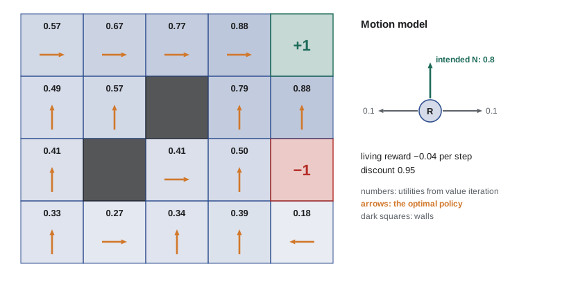
Our gridworld has 5 columns and 4 rows with two walls, a goal worth +1 in the top-right corner and a hazard worth −1 two squares below it. The robot's moves are unreliable: it goes the intended way with probability 0.8 and slips to each side with probability 0.1, staying put if it hits a wall. Every move costs 0.04 (a living reward of −0.04), and γ = 0.95.

# A gridworld MDP. The robot moves N, E, S or W; it goes the intended way with probability 0.8 and
# slips to each side with probability 0.1. Bumping into a wall or the edge leaves it in place.
W, H = 5, 4
WALLS = {(1, 1), (2, 2)}
TERMINAL = {(4, 3): +1.0, (4, 1): -1.0}
GAMMA = 0.95
MOVES = {"N": (0, 1), "E": (1, 0), "S": (0, -1), "W": (-1, 0)}
SIDES = {"N": "EW", "S": "EW", "E": "NS", "W": "NS"}
STATES = [(x, y) for y in range(H) for x in range(W) if (x, y) not in WALLS]

def step(s, a):
    nx, ny = s[0] + MOVES[a][0], s[1] + MOVES[a][1]
    return (nx, ny) if 0 <= nx < W and 0 <= ny < H and (nx, ny) not in WALLS else s

def outcomes(s, a):
    return [(0.8, step(s, a))] + [(0.1, step(s, side)) for side in SIDES[a]]

def show(values=None, policy=None):
    for y in reversed(range(H)):
        row = []
        for x in range(W):
            s = (x, y)
            if s in WALLS: row.append("  ####")
            elif s in TERMINAL: row.append(f"{TERMINAL[s]:+6.2f}" if values else f"{'+1' if TERMINAL[s] > 0 else '-1':>6}")
            elif values: row.append(f"{values[s]:6.3f}")
            else: row.append(f"{policy[s]:>6}")
        print("   " + " ".join(row))

def value_iteration(reward, eps=1e-6):
    U, sweeps = {s: 0.0 for s in STATES}, 0
    while True:
        sweeps += 1; delta = 0.0; new = {}
        for s in STATES:
            if s in TERMINAL: new[s] = TERMINAL[s]; continue
            new[s] = reward + GAMMA * max(sum(p * U[t] for p, t in outcomes(s, a)) for a in MOVES)   # Bellman update
            delta = max(delta, abs(new[s] - U[s]))
        U = new
        if delta < eps * (1 - GAMMA) / GAMMA: return U, sweeps

def greedy(U):
    return {s: max(MOVES, key=lambda a: sum(p * U[t] for p, t in outcomes(s, a))) for s in STATES if s not in TERMINAL}

U, sweeps = value_iteration(reward=-0.04)
print(f"value iteration converged after {sweeps} sweeps (living reward -0.04, gamma {GAMMA}); utilities:")
show(values=U)
print("optimal policy:")
show(policy=greedy(U))

value iteration converged after 32 sweeps (living reward -0.04, gamma 0.95); utilities:
    0.566  0.666  0.774  0.878  +1.00
    0.491  0.566   ####  0.785  0.878
    0.411   ####  0.412  0.501  -1.00
    0.329  0.265  0.335  0.389  0.178
optimal policy:
        E      E      E      E     +1
        N      N   ####      N      N
        N   ####      E      N     -1
        N      E      N      N      W

The utilities fall with distance from the goal and are lower near the hazard. The policy is interesting where risk matters. From the square directly below the hazard, the robot moves west, away from the hazard, rather than north toward the goal, because a slip while trying to pass the −1 square is costly. Next to the hazard on its left, the robot moves north, not east, because moving east would risk the hazard directly. The policy trades a slightly longer route for safety, exactly as maximizing expected utility requires.

Policy iteration

Policies often converge long before utilities do: the greedy policy stops changing even while the numbers are still settling. Policy iteration exploits this by alternating two steps. Policy evaluation computes the utility of every state under the current policy, which is a system of linear equations (no max), solvable exactly in O(n³) time or approximately by a few sweeps of simplified updates. Policy improvement then makes the policy greedy with respect to those utilities. When the improvement step changes nothing, the policy is optimal. Policy iteration usually needs only a handful of rounds.

The program below runs policy iteration with different living rewards, which shows how the reward function shapes behavior. With a small cost of living (−0.01), the robot is very cautious, taking long detours away from the hazard. As the cost rises, it accepts more risk to reach the goal sooner. With a living reward of −2.0, life is so painful that the robot heads straight for the nearest exit, even if that exit is the −1 hazard.

# A gridworld MDP. The robot moves N, E, S or W; it goes the intended way with probability 0.8 and
# slips to each side with probability 0.1. Bumping into a wall or the edge leaves it in place.
W, H = 5, 4
WALLS = {(1, 1), (2, 2)}
TERMINAL = {(4, 3): +1.0, (4, 1): -1.0}
GAMMA = 0.95
MOVES = {"N": (0, 1), "E": (1, 0), "S": (0, -1), "W": (-1, 0)}
SIDES = {"N": "EW", "S": "EW", "E": "NS", "W": "NS"}
STATES = [(x, y) for y in range(H) for x in range(W) if (x, y) not in WALLS]

def step(s, a):
    nx, ny = s[0] + MOVES[a][0], s[1] + MOVES[a][1]
    return (nx, ny) if 0 <= nx < W and 0 <= ny < H and (nx, ny) not in WALLS else s

def outcomes(s, a):
    return [(0.8, step(s, a))] + [(0.1, step(s, side)) for side in SIDES[a]]

def show(values=None, policy=None):
    for y in reversed(range(H)):
        row = []
        for x in range(W):
            s = (x, y)
            if s in WALLS: row.append("  ####")
            elif s in TERMINAL: row.append(f"{TERMINAL[s]:+6.2f}" if values else f"{'+1' if TERMINAL[s] > 0 else '-1':>6}")
            elif values: row.append(f"{values[s]:6.3f}")
            else: row.append(f"{policy[s]:>6}")
        print("   " + " ".join(row))

def evaluate(policy, reward, U, sweeps=30):
    for _ in range(sweeps):                       # simplified policy evaluation: repeated fixed-policy updates
        U = {s: TERMINAL[s] if s in TERMINAL else reward + GAMMA * sum(p * U[t] for p, t in outcomes(s, policy[s]))
             for s in STATES}
    return U

def policy_iteration(reward):
    policy = {s: "N" for s in STATES if s not in TERMINAL}
    U, rounds = {s: 0.0 for s in STATES}, 0
    while True:
        rounds += 1
        U = evaluate(policy, reward, U)
        new = {s: max(MOVES, key=lambda a: sum(p * U[t] for p, t in outcomes(s, a))) for s in policy}
        if new == policy: return policy, rounds
        policy = new

for reward in (-0.01, -0.04, -0.4, -2.0):
    policy, rounds = policy_iteration(reward)
    print(f"living reward {reward}: policy iteration stable after {rounds} rounds")
    show(policy=policy)

living reward -0.01: policy iteration stable after 4 rounds
        E      E      E      E     +1
        N      N   ####      N      N
        N   ####      E      N     -1
        N      W      N      N      W
living reward -0.04: policy iteration stable after 3 rounds
        E      E      E      E     +1
        N      N   ####      N      N
        N   ####      E      N     -1
        N      E      N      N      W
living reward -0.4: policy iteration stable after 3 rounds
        E      E      E      E     +1
        N      N   ####      N      N
        N   ####      E      N     -1
        N      E      E      N      N
living reward -2.0: policy iteration stable after 3 rounds
        E      E      E      E     +1
        N      N   ####      E      N
        N   ####      E      E     -1
        E      E      E      E      N

Policy iteration stabilizes in three or four rounds in every case, compared with 32 sweeps for value iteration to reach tight utilities. The policies differ in a few critical squares: compare the bottom row across the four outputs. The sensitivity of the optimal policy to the reward function is a reminder of lesson 1's warning: an agent faithfully optimizes the reward it is given, so the reward must say what we actually want.

Beyond fully observable MDPs

MDPs assume the agent always knows its state. When it does not, the problem becomes a partially observable MDP (POMDP). The agent must then act on a belief state, a probability distribution over states updated by Bayesian filtering after each action and observation, as in ROB-310's robot localization. A POMDP is equivalent to an MDP over belief states, but that space is continuous, and solving POMDPs exactly is intractable except for small problems; practical solvers use point-based approximations and online search. Optimal POMDP policies naturally include information-gathering actions, valued exactly as VPI suggests.

When the transition model and rewards are unknown, the agent must learn from experience: reinforcement learning. Methods such as temporal-difference learning and Q-learning estimate the Bellman quantities from sampled transitions instead of computing them from a model; combined with function approximation by neural networks, they produced TD-Gammon, the Atari-playing DQN agent and AlphaZero. AI-330 develops these methods.

Worked examples