Uninformed search

Many problems an agent faces have the same shape: it knows where it is, it knows what it wants, and it must find a sequence of actions that gets it there. Planning a road trip, solving a sliding-tile puzzle, sequencing the moves of a robot arm and finding a proof are all examples. This lesson shows how to formulate such problems precisely and how to solve them with search algorithms that use no knowledge beyond the problem definition itself. These uninformed (or blind) strategies are the baseline for everything that follows, and their costs, measured in nodes expanded and memory used, explain why lesson 3 needs heuristics.

CMPUT-204 covered breadth-first and depth-first traversal of explicit graphs, and Dijkstra's algorithm. The new element here is that the graph is usually implicit: it is defined by a start state and a function that generates successors, and it may be far too large to write down. The 8-puzzle has 181,440 reachable states, the 15-puzzle about ten trillion, and the state space of a delivery robot with a dozen parcels is larger still. A search algorithm explores only the part of the space it needs.

Formulating a problem

A search problem is defined by five components. Getting them right is often most of the work, because the formulation decides what the algorithm can and cannot find.

A solution is a sequence of actions from the initial state to a goal state; an optimal solution has the lowest path cost among all solutions. The formulation involves abstraction: we leave out the weather, the radio station and the exact position within a lane, keeping only what affects the choice of route. An abstraction is valid if every abstract solution can be expanded into a real one, and useful if carrying out the abstract actions is easier than the original problem.

The program below turns the 8-puzzle into code with exactly these components and then counts the state space. Breadth-first search outward from the goal reaches 181,440 states, exactly half of the 9! = 362,880 arrangements. The other half can never be reached, because every move preserves the parity of the permutation; this is why some scrambled 8-puzzles have no solution. The output also shows that the hardest instances need 31 moves.

# The 8-puzzle as a search problem, and the size of its state space.
from collections import deque
GOAL = (1, 2, 3, 4, 5, 6, 7, 8, 0)                  # 0 is the blank
MOVES = {"up": -3, "down": 3, "left": -1, "right": 1}

def actions(s):
    i = s.index(0); r, c = divmod(i, 3); acts = []
    if r > 0: acts.append("up")
    if r < 2: acts.append("down")
    if c > 0: acts.append("left")
    if c < 2: acts.append("right")
    return acts

def result(s, a):
    i = s.index(0); j = i + MOVES[a]; t = list(s)
    t[i], t[j] = t[j], t[i]
    return tuple(t)

# breadth-first search outward from the goal visits every reachable state once
depth, frontier = {GOAL: 0}, deque([GOAL])
while frontier:
    s = frontier.popleft()
    for a in actions(s):
        t = result(s, a)
        if t not in depth:
            depth[t] = depth[s] + 1; frontier.append(t)

counts = [0] * (max(depth.values()) + 1)
for d in depth.values(): counts[d] += 1
print("reachable states:", len(depth), "of 9! =", 362880)
print("hardest instances need", len(counts) - 1, "moves; there are", counts[-1], "of them")
print("states at each depth:", counts)

reachable states: 181440 of 9! = 362880
hardest instances need 31 moves; there are 2 of them
states at each depth: [1, 2, 4, 8, 16, 20, 39, 62, 116, 152, 286, 396, 748, 1024, 1893, 2512, 4485, 5638, 9529, 10878, 16993, 17110, 23952, 20224, 24047, 15578, 14560, 6274, 3910, 760, 221, 2]

Search trees, frontiers and repeated states

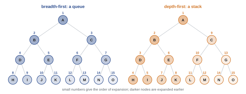
Search algorithms build a search tree. Its root is the initial state; expanding a node means applying every legal action to its state to generate child nodes. The frontier (sometimes called the open list) is the set of generated nodes that have not yet been expanded. Every algorithm in this lesson repeats the same loop: choose a node from the frontier, test whether it is a goal, and if not, expand it and add its children to the frontier. Algorithms differ only in which node they choose next.

A node is a bookkeeping structure: it holds a state, a pointer to its parent node, the action that generated it and the path cost from the root, g(n). Two different nodes can hold the same state if there are two paths to it. In a graph with cycles, a naive tree search can revisit states forever (Calgary to Banff to Calgary). Graph search fixes this by remembering every state it has reached and discarding new paths to them, unless (in cost-sensitive search) the new path is cheaper. The cost is memory: the reached set can hold every state seen. For the 8-puzzle the difference is dramatic, because almost every state can be reached by many move orders.

Measuring search algorithms

We judge a search algorithm on four criteria. Completeness asks whether it is guaranteed to find a solution when one exists. Optimality, also called admissibility, asks whether it finds a lowest-cost solution. Time complexity is usually measured by the number of nodes generated or expanded, and space complexity by the maximum number stored at once. Complexity is expressed in terms of the branching factor b (the maximum number of successors of any node), the depth d of the shallowest solution, the maximum depth m of the state space (which may be infinite) and, for uniform-cost search, the optimal cost C* and the smallest action cost ε.

Counting expanded nodes is a better measure than wall-clock time when comparing algorithms, because it does not depend on the computer, the language or how fast the successor function is. Throughout this course our programs print expansion counts so you can see the theory at work. The program below shows why exponential growth dominates everything: with b = 10, a fast search that generates a million nodes a second and stores a kilobyte per node runs out of memory long before it runs out of time.

# Time and memory for breadth-first search with branching factor b = 10,
# assuming 1 million nodes generated per second and 1 KB of memory per node.
def human(secs):
    for unit, size in (("years", 86400 * 365), ("days", 86400), ("hours", 3600), ("minutes", 60)):
        if secs >= size: return f"{secs / size:,.1f} {unit}"
    return f"{secs:.3g} seconds"
def mem(nbytes):
    for unit, size in (("TB", 1e12), ("GB", 1e9), ("MB", 1e6)):
        if nbytes >= size: return f"{nbytes / size:,.1f} {unit}"
    return f"{nbytes / 1e3:.1f} KB"
for d in (2, 4, 6, 8, 10, 12, 14, 16):
    nodes = sum(10 ** k for k in range(d + 1))
    print(f"depth {d:2}: {nodes:9.2e} nodes   time {human(nodes / 1e6):>17}   memory {mem(nodes * 1e3):>13}")

depth  2:  1.11e+02 nodes   time  0.000111 seconds   memory      111.0 KB
depth  4:  1.11e+04 nodes   time    0.0111 seconds   memory       11.1 MB
depth  6:  1.11e+06 nodes   time      1.11 seconds   memory        1.1 GB
depth  8:  1.11e+08 nodes   time       1.9 minutes   memory      111.1 GB
depth 10:  1.11e+10 nodes   time         3.1 hours   memory       11.1 TB
depth 12:  1.11e+12 nodes   time         12.9 days   memory    1,111.1 TB
depth 14:  1.11e+14 nodes   time         3.5 years   memory  111,111.1 TB
depth 16:  1.11e+16 nodes   time       352.3 years   memory 11,111,111.1 TB

Breadth-first search

Breadth-first search (BFS) expands the shallowest unexpanded node first, using a first-in, first-out queue as its frontier. It finds the solution with the fewest actions, and it is complete whenever b is finite. Because every node it generates must be kept (either on the frontier or in the reached set), its space complexity equals its time complexity, O(b^d). A useful trick is the early goal test: BFS can check whether a child is a goal as soon as it is generated rather than when it is expanded, saving a whole layer of work, because no later node can be shallower.

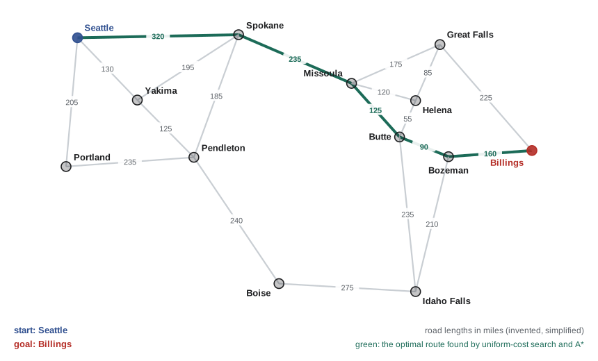
BFS is optimal only when every action has the same cost. On our road map, the route with the fewest roads is not the shortest drive.

# A simplified road map of the northwestern US (invented distances in miles, not official ones)
ROADS = [("Seattle", "Portland", 205), ("Seattle", "Yakima", 130), ("Seattle", "Spokane", 320),
         ("Portland", "Pendleton", 235), ("Yakima", "Pendleton", 125), ("Yakima", "Spokane", 195),
         ("Pendleton", "Boise", 240), ("Spokane", "Missoula", 235), ("Pendleton", "Spokane", 185),
         ("Boise", "Idaho Falls", 275), ("Missoula", "Butte", 125), ("Missoula", "Helena", 120),
         ("Missoula", "Great Falls", 175), ("Helena", "Great Falls", 85), ("Butte", "Helena", 55),
         ("Butte", "Bozeman", 90), ("Butte", "Idaho Falls", 235), ("Bozeman", "Billings", 160),
         ("Great Falls", "Billings", 225), ("Idaho Falls", "Bozeman", 210)]
COORDS = {"Seattle": (47.61, -122.33), "Portland": (45.52, -122.68), "Yakima": (46.60, -120.51),
          "Spokane": (47.66, -117.43), "Pendleton": (45.67, -118.79), "Boise": (43.62, -116.20),
          "Missoula": (46.87, -113.99), "Butte": (46.00, -112.53), "Helena": (46.59, -112.04),
          "Bozeman": (45.68, -111.04), "Idaho Falls": (43.49, -112.04), "Billings": (45.78, -108.50),
          "Great Falls": (47.50, -111.30)}
START, GOAL, UNIT, EARTH_R = "Seattle", "Billings", "mi", 3958.8

import math
GRAPH = {}
for a, b, d in ROADS:
    GRAPH.setdefault(a, []).append((b, d)); GRAPH.setdefault(b, []).append((a, d))
for city in GRAPH: GRAPH[city].sort()          # a fixed adjacency order makes runs repeatable
def straight_line(a, b):
    """Great-circle distance between two cities: never longer than any road between them."""
    (la1, lo1), (la2, lo2) = [(math.radians(x), math.radians(y)) for x, y in (COORDS[a], COORDS[b])]
    h = math.sin((la2 - la1) / 2) ** 2 + math.cos(la1) * math.cos(la2) * math.sin((lo2 - lo1) / 2) ** 2
    return 2 * EARTH_R * math.asin(math.sqrt(h))

from collections import deque
import heapq

def path_cost(path):
    return sum(dict(GRAPH[a])[b] for a, b in zip(path, path[1:]))

def bfs(start, goal):
    frontier, reached, expanded = deque([[start]]), {start}, 0
    while frontier:
        path = frontier.popleft(); expanded += 1
        for nxt, _ in GRAPH[path[-1]]:
            if nxt == goal: return path + [nxt], expanded      # early goal test
            if nxt not in reached:
                reached.add(nxt); frontier.append(path + [nxt])

def dfs(start, goal):
    frontier, expanded = [[start]], 0
    while frontier:
        path = frontier.pop()
        if path[-1] == goal: return path, expanded
        expanded += 1
        for nxt, _ in reversed(GRAPH[path[-1]]):
            if nxt not in path:                                # avoid cycles along the path
                frontier.append(path + [nxt])

def ucs(start, goal):
    frontier, best, expanded = [(0, [start])], {start: 0}, 0
    while frontier:
        g, path = heapq.heappop(frontier)
        if path[-1] == goal: return path, expanded             # late goal test
        if g > best[path[-1]]: continue                        # stale queue entry
        expanded += 1
        for nxt, d in GRAPH[path[-1]]:
            if g + d < best.get(nxt, float("inf")):
                best[nxt] = g + d; heapq.heappush(frontier, (g + d, path + [nxt]))

for name, f in [("breadth-first", bfs), ("depth-first", dfs), ("uniform-cost", ucs)]:
    path, n = f(START, GOAL)
    print(f"{name:14} expanded {n:2}  cost {path_cost(path):5} {UNIT}  {' > '.join(path)}")

breadth-first  expanded  9  cost   955 mi  Seattle > Spokane > Missoula > Great Falls > Billings
depth-first    expanded  6  cost  1325 mi  Seattle > Portland > Pendleton > Boise > Idaho Falls > Bozeman > Billings
uniform-cost   expanded 12  cost   930 mi  Seattle > Spokane > Missoula > Butte > Bozeman > Billings

Breadth-first search finds Seattle to Billings in four roads, via Spokane, Missoula and Great Falls, but that route is 955 miles. Uniform-cost search expands a few more nodes (12 rather than 9) and finds the 930 mile route through Butte and Bozeman. Depth-first search happens to expand few nodes here, but its route wanders south through Portland, Boise and Idaho Falls for 1,325 miles; it returned the first route it stumbled into.

Uniform-cost search

Uniform-cost search (UCS) expands the node with the lowest path cost g(n), using a priority queue. It is Dijkstra's algorithm, with two differences in emphasis: it stops when it removes a goal from the queue rather than computing distances to every node, and it generates the graph lazily. The goal test must be applied when a node is selected for expansion, not when it is generated, because a cheaper path to the goal might still be waiting in the queue. Our implementation uses the common lazy-deletion approach: when a cheaper path to a state is found, it pushes a new entry and skips stale entries when they surface.

UCS is complete and optimal provided every action cost is at least some ε > 0 (zero-cost cycles could trap it otherwise). Its complexity is not described naturally by d, because it explores in contours of equal cost; the bound is O(b^(1 + ⌊C*/ε⌋)), which can be much worse than BFS when many cheap actions lie around the start. When all costs are equal, UCS behaves like BFS but does a little more work because it waits to test the goal.

Depth-first search and its relatives

Depth-first search (DFS) expands the deepest node first, using a last-in, first-out stack (or recursion). Its virtue is memory: a tree-like DFS that checks for cycles only along the current path stores a single path plus the unexpanded siblings along it, O(bm) nodes. Its faults are serious. It is not optimal, and in an infinite state space, or one with cycles if it does not check them, it is not even complete: it can follow an infinite branch forever.

Depth-limited search fixes the infinite-path problem by treating nodes at a depth limit ℓ as if they had no successors. If we know a bound on the solution depth, for instance that any city on a map with 13 cities is reachable in at most 12 roads, we can use it. Usually we do not know a good limit, which motivates iterative deepening.

Iterative deepening search (IDS) runs depth-limited search with limits 0, 1, 2 and so on until it finds a goal. It looks wasteful, since shallow nodes are regenerated on every iteration, but in a tree with uniform branching most nodes are on the bottom level, so the repeated work is small. The total number of nodes generated is d·b + (d − 1)·b² + … + 1·b^d, which is O(b^d), the same order as BFS, while memory stays O(bd). For b = 10 and d = 5, IDS generates 123,450 nodes against BFS's 111,110, about 11 percent more, for an enormous saving in memory. IDS is the preferred uninformed method when the search space is large and the solution depth is unknown.

There is a catch, and the next experiment exposes it. That analysis assumes a tree. In a state space with many transpositions, where the same state is reached by many different paths, IDS without a reached set re-explores each state once for every path to it. On the 8-puzzle, BFS with a reached set expands several times fewer nodes than IDS at depth 18, though IDS still uses a tiny fraction of the memory. Choosing between them is a trade of time against memory.

# Breadth-first versus iterative deepening on 8-puzzle instances of known depth.
from collections import deque
import random
GOAL = (1, 2, 3, 4, 5, 6, 7, 8, 0)
ADJ = {i: [j for j in (i - 3, i + 3, i - 1, i + 1)
           if 0 <= j < 9 and (j // 3 == i // 3 or j % 3 == i % 3)] for i in range(9)}

def successors(s):
    i = s.index(0)
    for j in ADJ[i]:
        t = list(s); t[i], t[j] = t[j], t[i]; yield tuple(t)

def bfs(start):
    if start == GOAL: return 0, 0, 1
    frontier, parent, expanded, peak = deque([start]), {start: None}, 0, 1
    while frontier:
        s = frontier.popleft(); expanded += 1
        for t in successors(s):
            if t not in parent:
                parent[t] = s
                if t == GOAL:
                    n, u = 0, t
                    while parent[u] is not None: u, n = parent[u], n + 1
                    return n, expanded, max(peak, len(parent))
                frontier.append(t)
        peak = max(peak, len(parent))

def ids(start):
    expanded = 0
    def dls(s, limit, path):                       # depth-limited DFS, no repeats on the path
        nonlocal expanded
        if s == GOAL: return True
        if limit == 0: return False
        expanded += 1
        for t in successors(s):
            if t not in path:
                path.add(t)
                if dls(t, limit - 1, path): return True
                path.discard(t)
        return False
    for limit in range(40):
        if dls(start, limit, {start}): return limit, expanded, limit + 1

def scramble(k, rng):
    s, prev = GOAL, None
    for _ in range(k):
        options = [t for t in successors(s) if t != prev]
        prev, s = s, rng.choice(options)
    return s

rng = random.Random(366)
print("depth   BFS expanded  BFS memory   IDS expanded  IDS memory")
for k in (4, 8, 12, 14, 16, 18):
    s = scramble(k, rng)
    d1, e1, m1 = bfs(s); d2, e2, m2 = ids(s)
    assert d1 == d2
    print(f"{d1:5} {e1:14,} {m1:11,} {e2:14,} {m2:11,}")

depth   BFS expanded  BFS memory   IDS expanded  IDS memory
    4             11          23             19           5
    8            111         193            254           9
   12            709       1,108          2,009          13
   14          1,971       3,097          6,566          15
   16          4,897       7,521         18,931          17
   18         16,546      25,575         87,474          19

Bidirectional search

Bidirectional search runs two searches at once, one forward from the start and one backward from the goal, and stops when the frontiers meet. The motivation is arithmetic: b^(d/2) + b^(d/2) is far smaller than b^d. For b = 10 and d = 8, that is 20,000 nodes against 100 million. Bidirectional search needs a way to compute predecessors and a single explicit goal state (or a small set of them), which the 8-puzzle and route finding both have; it is harder to apply when the goal is described abstractly, such as 'any checkmate position'. Stopping correctly takes care: for optimal results the algorithm must finish the current layer, or for weighted graphs keep searching until the frontier costs guarantee no shorter connection remains.

# Bidirectional breadth-first search: grow one frontier from each end until they meet.
from collections import deque
import random
GOAL = (1, 2, 3, 4, 5, 6, 7, 8, 0)
ADJ = {i: [j for j in (i - 3, i + 3, i - 1, i + 1)
           if 0 <= j < 9 and (j // 3 == i // 3 or j % 3 == i % 3)] for i in range(9)}
def successors(s):
    i = s.index(0)
    for j in ADJ[i]:
        t = list(s); t[i], t[j] = t[j], t[i]; yield tuple(t)

def bfs_count(start):
    dist, q, expanded = {start: 0}, deque([start]), 0
    while q:
        s = q.popleft(); expanded += 1
        for t in successors(s):
            if t not in dist:
                dist[t] = dist[s] + 1
                if t == GOAL: return dist[t], expanded
                q.append(t)

def bidirectional(start):
    if start == GOAL: return 0, 0
    df, db = {start: 0}, {GOAL: 0}
    qf, qb, expanded = deque([start]), deque([GOAL]), 0
    while qf and qb:
        # expand one whole layer of the smaller frontier
        q, d, other = (qf, df, db) if len(qf) <= len(qb) else (qb, db, df)
        best = None
        for _ in range(len(q)):
            s = q.popleft(); expanded += 1
            for t in successors(s):
                if t in other:
                    cand = d[s] + 1 + other[t]
                    best = cand if best is None else min(best, cand)
                if t not in d:
                    d[t] = d[s] + 1; q.append(t)
        if best is not None: return best, expanded

rng = random.Random(4)
states = [GOAL]
for _ in range(60):                                 # a long random walk gives hard instances
    s = states[-1]; states.append(rng.choice(list(successors(s))))
for s in (states[20], states[40], states[60]):
    d1, e1 = bfs_count(s); d2, e2 = bidirectional(s)
    print(f"solution length {d1:2}: one-way BFS expanded {e1:7,}   bidirectional expanded {e2:6,}   same length: {d1 == d2}")

solution length  8: one-way BFS expanded      92   bidirectional expanded     30   same length: True
solution length 12: one-way BFS expanded     912   bidirectional expanded    102   same length: True
solution length 18: one-way BFS expanded  17,593   bidirectional expanded    605   same length: True

Comparing the strategies

None of these algorithms knows which direction the goal lies in. UCS expands nodes in all directions around the start, in growing rings of cost. On a map of North America, a search from Edmonton to Winnipeg using UCS would explore Vancouver and Kamloops almost as eagerly as Saskatoon, because it has no idea which way is east. Lesson 3 adds that knowledge in the form of a heuristic and shows how much it saves.

Worked examples