Local search and optimization

The algorithms of lessons 2 and 3 search for a path: the sequence of actions matters, and they keep the frontier and often every reached state in memory. In many problems, though, only the final configuration matters. An eight-queens arrangement, an exam timetable, a circuit layout or a delivery route is judged on its own merits, not by how we arrived at it. Local search algorithms keep a single current state (or a small population of states) and repeatedly move to a neighboring state, trying to improve an objective function. They use almost no memory and can handle state spaces far too large for systematic search, including continuous ones.

The price is that local search is usually incomplete: it may never find a solution even when one exists, and it rarely proves optimality. This lesson studies the basic algorithm, hill climbing, the ways it gets stuck, and three ways to escape: random restarts, simulated annealing and populations of states in local beam search and genetic algorithms. AI-430 treats derivative-free, evolutionary and convex optimization in depth; here we focus on the ideas and on measuring them.

The state-space landscape

Picture every state as a point on a landscape whose height is the objective value. If we are maximizing, the goal is the highest peak, the global maximum; if minimizing a cost, the lowest valley. A complete local search algorithm always finds a goal if one exists; an optimal one always finds a global optimum. Local search moves only between neighbors, states that differ by a small change such as moving one queen within its column or reversing a segment of a tour, so the shape of the landscape under that neighborhood decides how well it works.

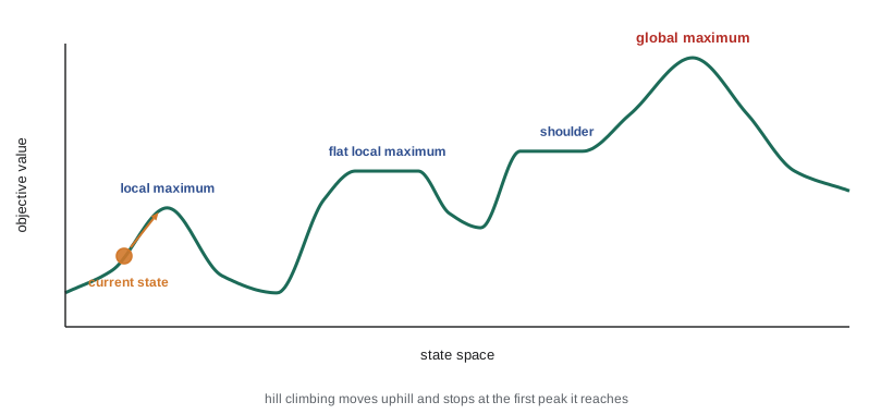
Three features of a landscape trap greedy algorithms. A local maximum is a peak higher than all its neighbors but lower than the global maximum; hill climbing that reaches one stops there. A plateau is a flat area where all neighbors have the same value: a flat local maximum from which no uphill exit exists, or a shoulder from which progress is possible after walking across. A ridge is a sequence of local maxima that rises gradually, but in a direction no single move follows, so every available move goes downhill. All three are common in practice.

Hill climbing

Hill climbing, also called greedy local search, is the simplest local search algorithm. From the current state it examines the neighbors and moves to the best one, stopping when no neighbor is better. In the steepest-ascent form it looks at every neighbor; in first-choice hill climbing it generates random neighbors and takes the first improvement, which is better when states have thousands of neighbors. Hill climbing does not look ahead beyond the immediate neighbors, which is why it is sometimes compared to climbing a mountain in thick fog with amnesia.

The eight-queens problem is a classic test. Place eight queens on a chessboard so that no two attack each other along a row, column or diagonal. In the complete-state formulation each column holds exactly one queen, so a state is a list of eight row numbers, and a neighbor moves one queen to another row of its column: 8 × 7 = 56 neighbors. The cost is the number of attacking pairs, and a solution has cost zero. Of the 16,777,216 possible states, 92 are solutions.

# Steepest-ascent hill climbing on 8-queens (one queen per column; the state gives each queen's row).
# Cost = number of attacking pairs; a solution has cost 0.
import random

def attacks(s):
    return sum(1 for i in range(8) for j in range(i + 1, 8)
               if s[i] == s[j] or abs(s[i] - s[j]) == j - i)

def hill_climb(s, rng, max_sideways=0):
    steps = sideways = 0
    while True:
        cost = attacks(s)
        if cost == 0: return True, steps
        best, moves = cost, []
        for col in range(8):
            for row in range(8):
                if row == s[col]: continue
                t = s[:col] + [row] + s[col + 1:]
                c = attacks(t)
                if c < best: best, moves = c, [t]
                elif c == best: moves.append(t)
        if best > cost or not moves: return False, steps        # local minimum
        if best == cost:                                         # plateau: allow a few sideways moves
            if sideways >= max_sideways: return False, steps
            sideways += 1
        else:
            sideways = 0
        s = rng.choice(moves); steps += 1

rng = random.Random(366)
starts = [[rng.randrange(8) for _ in range(8)] for _ in range(1000)]
rate = {}
for side in (0, 100):
    results = [hill_climb(list(s), random.Random(i), side) for i, s in enumerate(starts)]
    ok = [n for win, n in results if win]; bad = [n for win, n in results if not win]
    rate[side] = len(ok) / len(starts)
    print(f"sideways moves allowed {side:3}: solved {100 * rate[side]:.1f}% of 1000 starts;"
          f" mean steps {sum(ok) / len(ok):.1f} when solved, {sum(bad) / max(1, len(bad)):.1f} when stuck")
print(f"expected restarts until success without sideways moves: 1/p = {1 / rate[0]:.1f}")

sideways moves allowed   0: solved 13.6% of 1000 starts; mean steps 4.1 when solved, 3.1 when stuck
sideways moves allowed 100: solved 95.1% of 1000 starts; mean steps 19.3 when solved, 59.7 when stuck
expected restarts until success without sideways moves: 1/p = 7.4

Plain hill climbing solves only about 14 percent of random starts, and it fails fast: about three steps before getting stuck in a local minimum, and about four steps when it succeeds. Allowing up to 100 consecutive sideways moves (moves to an equally good neighbor) lets it cross plateaus, raising the success rate to about 95 percent at the cost of about 20 steps per success. Plateaus, not true local minima, are the main obstacle on this landscape.

Random-restart hill climbing is the simplest fix for getting stuck: if a run fails, start again from a new random state. If each run succeeds with probability p, the expected number of runs is 1/p, about 7 for plain hill climbing on eight-queens, so the expected total is roughly 7 × 3 + 4, under 30 steps. Random restarts make hill climbing complete with probability approaching 1, since eventually a start lands in the basin of a global optimum. The method works remarkably well on many problems, and lesson 6 shows a close relative, min-conflicts, solving n-queens with a thousand queens in a few dozen moves.

Simulated annealing

Hill climbing never moves downhill, so it can get stuck; a purely random walk eventually finds anything but is hopelessly slow. Simulated annealing combines them. It picks a random neighbor; if the move improves the objective, it always accepts it; if the move makes things worse by Δ, it accepts it with probability

where T, the temperature, starts high and decreases according to a cooling schedule. At high temperature, bad moves are often accepted and the search roams the landscape; as T falls, the search becomes increasingly greedy and settles into a deep valley. The name comes from metallurgy: annealing heats metal and cools it slowly so that its atoms settle into a low-energy crystalline arrangement. Kirkpatrick, Gelatt and Vecchi introduced the method for chip layout in 1983. If the temperature is lowered slowly enough, the probability of ending in a global optimum approaches 1, though the schedule needed for that guarantee is usually impractically slow.

The traveling salesperson problem (TSP) asks for the shortest tour visiting every city once and returning home. It is NP-hard, and it is a natural fit for local search. The standard neighborhood is 2-opt: remove two edges of the tour and reconnect the two paths the other way, which amounts to reversing a segment. The program compares a constructive heuristic (nearest neighbor), 2-opt hill climbing from random tours, and simulated annealing using the same 2-opt moves, on 40 seeded random cities.

# The TSP on 40 random cities: nearest city first, 2-opt hill climbing and simulated annealing.
import math, random
rng = random.Random(366)
N = 40
pts = [(rng.random() * 100, rng.random() * 100) for _ in range(N)]
D = [[math.dist(a, b) for b in pts] for a in pts]
def length(t): return sum(D[t[i]][t[i - 1]] for i in range(len(t)))

def nearest_first():
    tour, left = [0], set(range(1, N))
    while left:
        nxt = min(left, key=lambda j: (D[tour[-1]][j], j)); tour.append(nxt); left.remove(nxt)
    return tour

def two_opt_delta(t, i, j):
    """Change in length from reversing t[i..j]."""
    a, b, c, d = t[i - 1], t[i], t[j], t[(j + 1) % N]
    return D[a][c] + D[b][d] - D[a][b] - D[c][d]

def hill_climb_2opt(t):
    improved = True
    while improved:
        improved = False
        for i in range(1, N - 1):
            for j in range(i + 1, N):
                if two_opt_delta(t, i, j) < -1e-12:
                    t[i:j + 1] = reversed(t[i:j + 1]); improved = True
    return t

def anneal(t, rng, T0=20.0, T_end=0.05, steps=100000):
    alpha = (T_end / T0) ** (1 / steps)                      # geometric cooling schedule
    best, best_len, cur_len, T = t[:], length(t), length(t), T0
    for _ in range(steps):
        i = rng.randrange(1, N - 1); j = rng.randrange(i + 1, N)
        delta = two_opt_delta(t, i, j)
        if delta < 0 or rng.random() < math.exp(-delta / T):   # sometimes accept a worse tour
            t[i:j + 1] = reversed(t[i:j + 1]); cur_len += delta
            if cur_len < best_len: best, best_len = t[:], cur_len
        T *= alpha
    return best

start = list(range(N)); random.Random(1).shuffle(start)
print(f"random tour             {length(start):7.1f}")
print(f"nearest-city tour       {length(nearest_first()):7.1f}")
hc = [length(hill_climb_2opt(random.Random(s).sample(range(N), N))) for s in range(10)]
print(f"2-opt hill climbing     {min(hc):7.1f} best of 10 restarts, mean {sum(hc) / 10:.1f}")
sa = [length(anneal(random.Random(s).sample(range(N), N), random.Random(s))) for s in range(10)]
print(f"simulated annealing     {min(sa):7.1f} best of 10 runs,     mean {sum(sa) / 10:.1f}")

random tour              2214.5
nearest-city tour         603.0
2-opt hill climbing       536.2 best of 10 restarts, mean 560.7
simulated annealing       536.2 best of 10 runs,     mean 538.6

The nearest-neighbor heuristic, which always drives to the closest unvisited city, quickly builds a tour about 12 percent longer than the best found. Ten 2-opt hill-climbing runs average about 561, with the best run reaching 536.2. Simulated annealing averages about 539 and reaches the same best tour in several runs. The best tour is probably optimal, but local search cannot tell us so; proving optimality would take an exact method such as branch and bound or integer programming. Production TSP solvers such as Concorde and LKH combine powerful local search moves (Lin–Kernighan) with exact bounds and have solved instances with tens of thousands of cities to proven optimality.

Tuning matters. The starting temperature should accept most bad moves at first, the final temperature should accept almost none, and the number of steps controls the quality. Our run cools geometrically from T = 20 to T = 0.05 over 100,000 steps. Too-fast cooling makes annealing a slower version of hill climbing; too-slow cooling wastes time. In practice annealing is often run with a fixed time budget and the best state seen is returned.

Local beam search

Local beam search keeps k states instead of one. At each step it generates all the successors of all k states and keeps the best k of the whole pool. This is not the same as k independent restarts: if one state generates several good successors, the search concentrates there, passing useful information between the parallel threads. The danger is lack of diversity, as all k states can crowd onto one small hill. Stochastic beam search chooses the k successors at random, with probability increasing with their value, which keeps some diversity. Beam search is also the standard decoding method for many sequence models, where k partial outputs are kept at each step.

Genetic algorithms

A genetic algorithm is a stochastic beam search in which successors are produced by combining two parent states rather than modifying one. It keeps a population of individuals, each encoded as a string (for eight-queens, the eight row numbers). Each generation selects parents with probability favoring higher fitness, produces children by crossover (taking a prefix from one parent and the suffix from the other) and applies random mutation to a few positions. Elitism copies the best individuals unchanged into the next generation so that the best fitness never decreases.

# A genetic algorithm for 8-queens. Fitness = number of non-attacking pairs (28 is perfect).
import random

def fitness(s):
    return 28 - sum(1 for i in range(8) for j in range(i + 1, 8)
                    if s[i] == s[j] or abs(s[i] - s[j]) == j - i)

def evolve(rng, size=100, rate=0.1, k=3, limit=500, trace=False):
    pop = [[rng.randrange(8) for _ in range(8)] for _ in range(size)]
    for gen in range(limit):
        best = max(pop, key=fitness)
        if trace and (gen % 5 == 0 or fitness(best) == 28):
            print(f"  generation {gen:3}: best {fitness(best)}  mean {sum(map(fitness, pop)) / size:.1f}  {best}")
        if fitness(best) == 28: return gen
        select = lambda: max(rng.sample(pop, k), key=fitness)       # tournament of k
        children = [best]                                           # elitism: keep the best
        while len(children) < size:
            a, b = select(), select()
            cut = rng.randrange(1, 8)                               # one-point crossover
            child = [rng.randrange(8) if rng.random() < rate else g for g in a[:cut] + b[cut:]]
            children.append(child)
        pop = children
    return None

print("one run (seed 6):")
evolve(random.Random(6), trace=True)
gens = [evolve(random.Random(seed)) for seed in range(20)]
solved = sorted(g for g in gens if g is not None)
print(f"20 runs: solved {len(solved)} within 500 generations; median {solved[len(solved) // 2]} generations")

one run (seed 6):
  generation   0: best 25  mean 19.9  [6, 5, 1, 1, 6, 0, 3, 7]
  generation   5: best 26  mean 21.7  [7, 6, 4, 1, 5, 0, 2, 3]
  generation  10: best 26  mean 22.9  [7, 6, 4, 1, 5, 0, 2, 3]
  generation  15: best 28  mean 23.6  [3, 6, 4, 1, 5, 0, 2, 7]
20 runs: solved 18 within 500 generations; median 18 generations

With a population of 100, the genetic algorithm usually solves eight-queens within a few dozen generations (the median over 20 seeds is 18), but two of the 20 seeded runs did not finish within 500 generations: the population converged on a near-solution and mutation alone failed to escape. Premature convergence is the central practical difficulty with genetic algorithms. Crossover helps only when the encoding puts related decisions in contiguous blocks, so that a good block from one parent can combine with a good block from another; for eight-queens, a prefix of columns that is free of attacks is such a block. When there is no such structure, a genetic algorithm is typically no better than simulated annealing or restarts. Genetic algorithms and their relatives in evolutionary computation have produced useful designs, including a NASA spacecraft antenna, and remain common for hard optimization problems with awkward objectives.

Local search in continuous spaces

Many real problems have continuous variables: where to place a depot, the angles of a robot arm, the weights of a neural network. A continuous state has infinitely many neighbors, so we cannot enumerate them. If the objective is differentiable, the gradient points in the direction of steepest increase, and gradient descent (for minimization) takes steps x ← x − α∇f(x). The step size α matters: too large and the search overshoots; too small and it crawls. A line search, which shrinks the step whenever it fails to improve, is a simple robust choice. Newton's method uses second derivatives to choose both direction and step, converging much faster near an optimum at a higher cost per step.

# Local search in a continuous space: place one depot to minimize the total distance to six towns
# (the Weber problem). Gradient descent with a shrinking step size.
import math
towns = [(0, 0), (40, 10), (90, 0), (60, 70), (20, 80), (85, 95)]
def cost(x, y): return sum(math.hypot(x - a, y - b) for a, b in towns)
def grad(x, y):
    gx = gy = 0.0
    for a, b in towns:
        r = math.hypot(x - a, y - b) or 1e-9
        gx += (x - a) / r; gy += (y - b) / r
    return gx, gy

x, y = sum(a for a, _ in towns) / 6, sum(b for _, b in towns) / 6     # start at the centroid
print(f"centroid      ({x:5.1f}, {y:5.1f})  total distance {cost(x, y):.2f}")
step = 5.0
for it in range(1, 201):
    gx, gy = grad(x, y)
    nx, ny = x - step * gx, y - step * gy
    if cost(nx, ny) < cost(x, y): x, y = nx, ny                     # accept only improvements
    else: step /= 2                                                  # otherwise take smaller steps
    if it in (1, 5, 20, 200): print(f"iteration {it:3} ({x:5.1f}, {y:5.1f})  total distance {cost(x, y):.2f}  step {step:.4f}")

centroid      ( 49.2,  42.5)  total distance 298.32
iteration   1 ( 49.1,  43.5)  total distance 298.13  step 5.0000
iteration   5 ( 49.4,  46.1)  total distance 297.81  step 5.0000
iteration  20 ( 49.9,  48.2)  total distance 297.71  step 5.0000
iteration 200 ( 50.0,  48.3)  total distance 297.71  step 0.0000

The centroid minimizes the sum of squared distances, not the sum of distances, so gradient descent improves on it, moving the depot north to a point that is about 0.6 units better in total distance. This objective is convex, so the local optimum found is also the global one. Most objectives of interest are not convex, and continuous local search then has the same local-optimum problem as discrete hill climbing, handled with the same ideas: restarts, randomness and momentum. Training a neural network is local search in a space with millions or billions of dimensions; AI-420 and AI-430 study those methods.

Worked examples