Shortest paths revisited: Bellman–Ford, Floyd–Warshall and Johnson

CMPUT-204 presented Dijkstra's algorithm for nonnegative edge weights and Bellman–Ford for weights that may be negative, including the detection of negative cycles. This lesson looks at both again through the lens of dynamic programming, which explains why Bellman–Ford works and how many rounds it needs, and then turns to the all-pairs problem: computing the shortest distance between every pair of vertices. Floyd–Warshall solves it with a short triple loop whose correctness rests on a clever choice of subproblem, and Johnson's algorithm combines one run of Bellman–Ford with many runs of Dijkstra by reweighting the edges so that none is negative. Negative weights are not exotic: they arise from rebates and credits, from logarithms of exchange rates, and from reductions such as the difference constraints used in scheduling.

Bellman–Ford as a dynamic program

Let \(d_i(v)\) be the length of a shortest walk from s to v that uses at most i edges, or \(\infty\) if there is none. A walk with at most i edges either uses at most \(i - 1\) edges, or its last edge is some \((u, v)\) and the rest is a walk to u with at most \(i - 1\) edges. So \(d_i(v) = \min(d_{i-1}(v),\ \min_{(u,v) \in E} (d_{i-1}(u) + w(u, v)))\), with \(d_0(s) = 0\) and \(d_0(v) = \infty\) otherwise. This is exactly the recipe of lesson 2, with 'number of edges allowed' as the extra index. If the graph has no negative cycle, some shortest path is simple and so uses at most \(n - 1\) edges, so \(d_{n-1}(v)\) is the true distance. Each round examines every edge once, giving \(O(nm)\) time and, if only the previous round is kept, \(O(n)\) space.

# Bellman-Ford as dynamic programming: d_i(v) = shortest s-v walk using at most i edges.
# d_i(v) = min(d_{i-1}(v), min over edges (u, v) of d_{i-1}(u) + w(u, v)).
INF = float("inf")
V = ["s", "a", "b", "c", "d", "t"]
E = [("s", "a", 4), ("s", "b", 2), ("b", "a", 1), ("a", "c", 2), ("b", "c", 6),
     ("c", "d", -4), ("b", "d", 3), ("d", "t", 2), ("c", "t", 5), ("a", "t", 9)]

d = {v: INF for v in V}; d["s"] = 0
pred = {v: None for v in V}
print("round " + "".join(f"{v:>5}" for v in V))
print(f"{0:5d} " + "".join(f"{d[v]:>5}" for v in V))
for i in range(1, len(V)):
    new = dict(d)
    for u, v, w in E:                      # use only round i-1 values: the textbook DP
        if d[u] + w < new[v]:
            new[v] = d[u] + w; pred[v] = u
    changed = new != d
    d = new
    print(f"{i:5d} " + "".join(f"{d[v]:>5}" for v in V))
    if not changed:
        print("no change: stop early"); break
path, x = [], "t"
while x: path.append(x); x = pred[x]
print("shortest s-t path:", " -> ".join(reversed(path)), "length", d["t"])

round     s    a    b    c    d    t
    0     0  inf  inf  inf  inf  inf
    1     0    4    2  inf  inf  inf
    2     0    3    2    6    5   13
    3     0    3    2    5    2    7
    4     0    3    2    5    1    4
    5     0    3    2    5    1    3
shortest s-t path: s -> b -> a -> c -> d -> t length 3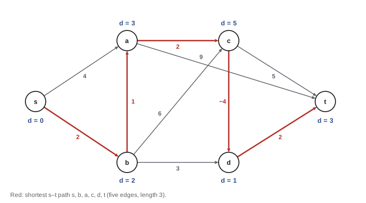

Real implementations relax edges in place, using values from the current round as soon as they are available. That can only make distances smaller sooner, and it never makes them wrong, because every value is always the length of some real walk. Two further practical improvements are to stop as soon as a round changes nothing, and to relax only edges leaving vertices whose distance changed in the previous round (a queue-based variant often called SPFA). Neither improves the \(O(nm)\) worst case.

Negative cycles

If some cycle reachable from s has negative total weight, walks can be made arbitrarily short by going around it, and shortest paths are no longer well defined by this method. Bellman–Ford detects the situation: if after \(n - 1\) rounds some edge can still be relaxed, a negative cycle exists, because without one the values would already be final. To find the cycle, note that the predecessor pointers then contain a cycle. Starting from the vertex just relaxed and following predecessors n times is guaranteed to land on the cycle, and walking around it from there lists its vertices. Adding a virtual source with zero-weight edges to every vertex makes every cycle reachable, so the method finds a negative cycle anywhere in the graph.

Currency exchange is the classic illustration. If converting a unit of currency a into currency b yields \(r_{ab}\) units, a sequence of conversions that returns to the start with more money than it began with is an arbitrage. Its product of rates exceeds 1 exactly when the sum of \(-\log r_{ab}\) is negative, so arbitrage is a negative cycle in the graph with weights \(-\log r_{ab}\). The program below uses invented rates chosen to contain one such cycle.

# Detecting and extracting a negative cycle: if any edge can still be relaxed after
# n - 1 rounds, follow predecessors n times to land on the cycle, then walk around it.
def negative_cycle(V, E):
    d = {v: 0 for v in V}                  # a virtual source joined to every vertex by weight 0
    pred = {v: None for v in V}
    for _ in range(len(V) - 1):
        for u, v, w in E:
            if d[u] + w < d[v]: d[v] = d[u] + w; pred[v] = u
    for u, v, w in E:
        if d[u] + w < d[v]:
            pred[v] = u
            x = v
            for _ in range(len(V)): x = pred[x]          # now x is on a cycle
            cyc, y = [x], pred[x]
            while y != x: cyc.append(y); y = pred[y]
            return cyc[::-1]
    return None

# Exchange rates between five currencies (illustrative numbers, not market data).
import math
rates = {("CAD", "USD"): 0.73, ("USD", "EUR"): 0.92, ("EUR", "GBP"): 0.86,
         ("GBP", "CAD"): 1.75, ("USD", "JPY"): 150.0, ("JPY", "CAD"): 0.0091,
         ("EUR", "CAD"): 1.46}
V = sorted({c for pair in rates for c in pair})
E = [(a, b, -math.log(r)) for (a, b), r in rates.items()]   # product > 1  <=>  sum of -log < 0
cyc = negative_cycle(V, E)
print("negative cycle:", " -> ".join(cyc + [cyc[0]]))
prod = 1.0
for a, b in zip(cyc, cyc[1:] + cyc[:1]): prod *= rates[(a, b)]
print(f"one unit around the cycle becomes {prod:.4f} units")

negative cycle: USD -> EUR -> GBP -> CAD -> USD
one unit around the cycle becomes 1.0108 units

All pairs: Floyd–Warshall

Aspen Valley's planners want a table of shortest driving times between every pair of its depots, customers and transfer points. Running Bellman–Ford from every vertex costs \(O(n^2 m)\), which is \(O(n^4)\) for dense graphs. Floyd–Warshall, published by Floyd and by Warshall in 1962 (Roy had a version in 1959), takes \(O(n^3)\) time with a much smaller constant. Number the vertices 1 to n. Let \(D_k[i][j]\) be the length of a shortest path from i to j whose intermediate vertices all lie in \(\{1, \dots, k\}\). For \(k = 0\) no intermediate vertices are allowed, so \(D_0[i][j]\) is the edge weight, 0 on the diagonal and \(\infty\) if there is no edge.

Recurrence. A shortest path from i to j with intermediates in \(\{1, \dots, k\}\) either does not use k, and then has length \(D_{k-1}[i][j]\), or uses k exactly once (with no negative cycles, a shortest path is simple), and then splits into a path from i to k and a path from k to j, each with intermediates in \(\{1, \dots, k-1\}\). Hence \(D_k[i][j] = \min(D_{k-1}[i][j],\ D_{k-1}[i][k] + D_{k-1}[k][j])\). The answer is \(D_n\). The table at step k needs only the table at step \(k - 1\), and since \(D_k[i][k] = D_{k-1}[i][k]\) and \(D_k[k][j] = D_{k-1}[k][j]\), the update can be done in place in a single \(n \times n\) array. A negative diagonal entry at the end signals a negative cycle.

# Floyd-Warshall: D_k[i][j] = shortest i-j path whose intermediate vertices are among 0..k-1.
INF = float("inf")
names = ["depot", "mall", "farm", "mill", "lake"]
n = len(names)
w = {(0, 1): 7, (0, 2): 3, (2, 1): 2, (1, 3): 4, (2, 3): 8, (3, 4): 1, (4, 0): 6, (2, 4): 9, (4, 2): -2}
D = [[0 if i == j else w.get((i, j), INF) for j in range(n)] for i in range(n)]
nxt = [[j if (i, j) in w else None for j in range(n)] for i in range(n)]
for k in range(n):
    for i in range(n):
        for j in range(n):
            if D[i][k] + D[k][j] < D[i][j]:
                D[i][j] = D[i][k] + D[k][j]; nxt[i][j] = nxt[i][k]
assert all(D[i][i] >= 0 for i in range(n)), "negative cycle"
print("       " + "".join(f"{x:>7}" for x in names))
for i in range(n):
    print(f"{names[i]:>7}" + "".join(f"{D[i][j]:>7}" for j in range(n)))
def path(i, j):
    p = [i]
    while i != j: i = nxt[i][j]; p.append(i)
    return " -> ".join(names[x] for x in p)
print("depot to lake:", path(0, 4), "=", D[0][4])
print("lake to mall: ", path(4, 1), "=", D[4][1])

         depot   mall   farm   mill   lake
  depot      0      5      3      9     10
   mall     11      0      3      4      5
   farm     13      2      0      6      7
   mill      7      1     -1      0      1
   lake      6      0     -2      4      0
depot to lake: depot -> farm -> mall -> mill -> lake = 10
lake to mall:  lake -> farm -> mall = 0

The choice of subproblem is what makes this work. A tempting alternative, 'shortest path from i to j using at most k edges', gives the repeated-squaring algorithm of \(O(n^3 \log n)\) time, which is worse. Restricting which vertices may be used in the middle of a path lets each step add exactly one new vertex and consider it once. Replacing min and plus by 'or' and 'and' turns the same triple loop into Warshall's algorithm for the transitive closure of a relation: which vertices can reach which.

Johnson's algorithm for sparse graphs

For sparse graphs, n runs of Dijkstra with a binary heap take \(O(nm \log n)\) time, far less than \(n^3\) when m is close to n. But Dijkstra fails with negative weights. Johnson's 1977 idea is to reweight the edges so that all weights become nonnegative while shortest paths stay the same. Choose any function h on vertices, a potential, and set \(w'(u, v) = w(u, v) + h(u) - h(v)\). For any path \(v_0, v_1, \dots, v_k\), the new length telescopes: \(\sum w'(v_{i-1}, v_i) = \sum w(v_{i-1}, v_i) + h(v_0) - h(v_k)\). Every path between the same two endpoints changes by the same amount, so shortest paths are preserved, and distances are recovered by subtracting \(h(v_0) - h(v_k)\).

To make the new weights nonnegative, add a new vertex q with zero-weight edges to every vertex and let \(h(v)\) be the shortest distance from q to v, computed by one run of Bellman–Ford. The triangle inequality for shortest distances, \(h(v) \le h(u) + w(u, v)\), says precisely that \(w'(u, v) \ge 0\). The total time is \(O(nm)\) for Bellman–Ford plus \(O(nm \log n)\) for the Dijkstra runs. If Bellman–Ford finds a negative cycle, the algorithm reports it instead.

# Johnson's algorithm: Bellman-Ford once to get potentials h, reweight
# w'(u, v) = w(u, v) + h(u) - h(v) >= 0, then Dijkstra from every vertex.
import heapq
INF = float("inf")
n = 5
w = {(0, 1): 7, (0, 2): 3, (2, 1): 2, (1, 3): 4, (2, 3): 8, (3, 4): 1, (4, 0): 6, (2, 4): 9, (4, 2): -2}

h = [0] * n                                    # virtual source q with 0-weight edges to all
for _ in range(n):
    for (u, v), c in w.items():
        h[v] = min(h[v], h[u] + c)
wp = {(u, v): c + h[u] - h[v] for (u, v), c in w.items()}
print("potentials h:", h)
print("smallest reweighted edge:", min(wp.values()))

def dijkstra(src):
    dist = [INF] * n; dist[src] = 0; pq = [(0, src)]
    while pq:
        d, u = heapq.heappop(pq)
        if d > dist[u]: continue
        for (a, b), c in wp.items():
            if a == u and d + c < dist[b]:
                dist[b] = d + c; heapq.heappush(pq, (dist[b], b))
    return dist

D = [[dijkstra(u)[v] - h[u] + h[v] for v in range(n)] for u in range(n)]   # undo the reweighting
for row in D: print(row)

potentials h: [0, 0, -2, 0, 0]
smallest reweighted edge: 0
[0, 5, 3, 9, 10]
[11, 0, 3, 4, 5]
[13, 2, 0, 6, 7]
[7, 1, -1, 0, 1]
[6, 0, -2, 4, 0]

Which algorithm when

# Rough operation counts for all-pairs shortest paths on sparse and dense graphs.
import math
print(f"{'n':>6} {'m':>9}  {'n * Bellman-Ford':>18}  {'Floyd-Warshall':>15}  {'Johnson':>15}")
for n, m in ((1000, 4000), (1000, 400000), (10000, 40000), (10000, 10 ** 7)):
    bf = n * n * m
    fw = n ** 3
    jo = n * m + n * (m + n) * math.log2(n)
    print(f"{n:>6} {m:>9}  {bf:>18.2e}  {fw:>15.2e}  {jo:>15.2e}")

     n         m    n * Bellman-Ford   Floyd-Warshall          Johnson
  1000      4000            4.00e+09         1.00e+09         5.38e+07
  1000    400000            4.00e+11         1.00e+09         4.40e+09
 10000     40000            4.00e+12         1.00e+12         7.04e+09
 10000  10000000            1.00e+15         1.00e+12         1.43e+12

Shortest paths remain an active research area. In 2022 Bernstein, Nanongkai and Wulff-Nilsen gave a randomized algorithm for single-source shortest paths with negative integer weights in nearly linear time, and in 2025 Duan and coauthors showed that directed single-source shortest paths with nonnegative real weights can be computed faster than sorting, breaking a barrier that Dijkstra's algorithm had seemed to set. These algorithms are intricate and not yet the ones used in practice, but they show that even a problem studied since the 1950s still holds surprises.

Worked examples