Why algorithms II: from efficient algorithms to hard problems

CMPUT-204 gave you a toolkit for designing efficient algorithms and proving them correct: asymptotic analysis, recurrences, divide and conquer, greedy choices with exchange arguments, graph search, shortest paths and minimum spanning trees. Many problems yield to those tools. Many do not. Some need a more systematic way to reuse the answers to overlapping subproblems; that is dynamic programming. Some ask for the best way to route material through a network, or to pair up two kinds of objects; those need network flow and its close relative, linear programming. And some problems seem to resist every technique. For those we need a theory that explains why, so that we stop looking for an algorithm that probably does not exist and start looking for the next best thing.

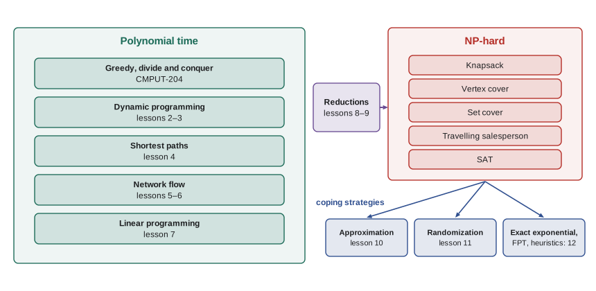
This course follows that arc. Lessons 2 to 7 add three powerful design techniques: dynamic programming, network flow and linear programming with duality. Lessons 8 and 9 introduce the theory of NP-completeness, which lets you prove that a problem is as hard as a large family of problems that nobody has solved efficiently in more than fifty years of trying. Lessons 10 to 12 show what to do next: approximation algorithms with proven guarantees, randomized algorithms that trade certainty for speed and simplicity, and exact algorithms that are exponential but much faster than brute force. CMPUT-474 later treats the same complexity classes from the side of formal models and Turing machines; here the emphasis is on designing algorithms and on reductions as a working tool.

A running case: Aspen Valley Couriers

The capstone of CMPUT-204 introduced Aspen Valley Couriers, an invented regional delivery company with a depot, a fleet of vans and a few dozen drivers. Its daily problems keep turning up in this course. How should the dispatcher choose which parcels go in a van with a weight limit so that the value delivered is as large as possible? That is a knapsack problem, solved by dynamic programming in lesson 3. Which pairs of drivers and vans should be assigned when each driver is licensed for only some vehicles? That is bipartite matching, solved by flow in lesson 6. In what order should a van visit its stops? That is the traveling salesperson problem, NP-hard, and the subject of approximation in lesson 10 and of heuristics in lesson 12. Each time, the first question is the same: which kind of problem is this?

Look-alike problems with very different difficulty

A recurring surprise in algorithms is that two problems that sound almost identical can sit on opposite sides of the efficiency boundary. Consider a delivery van that must drive along every street of a neighborhood exactly once, for example to inspect road surfaces, and return to the depot. Model the streets as edges of a graph. Euler proved in 1736 that such a closed walk, an Euler circuit, exists in a connected graph exactly when every vertex has even degree. The test takes linear time, and Hierholzer's algorithm constructs the circuit in linear time as well. Now change one word: the van must visit every intersection exactly once and return. This is a Hamiltonian cycle, and no polynomial-time algorithm is known for deciding whether one exists. The best known exact algorithms take exponential time in the worst case.

# Two look-alike problems: use every EDGE once (Euler) or every VERTEX once (Hamilton).
# Euler has a linear-time test; for Hamilton we only know exponential search in general.
from itertools import permutations
import random
random.seed(304)

def euler_circuit(n, edges):
    deg = [0] * n
    adj = {v: set() for v in range(n)}
    for u, v in edges:
        deg[u] += 1; deg[v] += 1; adj[u].add(v); adj[v].add(u)
    start = next(v for v in range(n) if deg[v])
    seen, stack = {start}, [start]
    while stack:                                  # one graph search: O(n + m) steps
        x = stack.pop()
        for y in adj[x]:
            if y not in seen:
                seen.add(y); stack.append(y)
    ok = all(deg[v] == 0 or v in seen for v in range(n)) and all(d % 2 == 0 for d in deg)
    return ok, n + len(edges)

def hamilton_cycle(n, edges):
    E = {frozenset(e) for e in edges}
    checked = 0
    for p in permutations(range(1, n)):           # fix vertex 0, try every order of the rest
        checked += 1
        cyc = (0,) + p
        if all(frozenset((cyc[i], cyc[(i + 1) % n])) in E for i in range(n)):
            return True, checked
    return False, checked

print(" n  edges  Euler?  steps   Hamilton?  orders checked")
for n in (6, 8, 10):
    edges = set()
    while len(edges) < int(1.6 * n):
        u, v = random.sample(range(n), 2)
        edges.add((min(u, v), max(u, v)))
    edges = sorted(edges)
    e, s1 = euler_circuit(n, edges)
    h, s2 = hamilton_cycle(n, edges)
    print(f"{n:2d}  {len(edges):5d}  {e!s:6s}  {s1:5d}   {h!s:9s}  {s2:14d}")

 n  edges  Euler?  steps   Hamilton?  orders checked
 6      9  False      15   True                   61
 8     12  False      20   True                  120
10     16  False      26   False              362880

The output shows the pattern even on tiny random graphs. The Euler test touches each vertex and edge a constant number of times. The Hamilton search sometimes stops early when it is lucky, but when no cycle exists it must check every one of the \((n-1)!\) orders. Clever pruning helps, and lesson 12 shows a dynamic program that runs in \(O(2^n n^2)\) time instead of \(O(n!)\), but nobody knows an algorithm that is polynomial in n.

Other pairs behave the same way. Shortest paths can be found in polynomial time even with negative edge weights, provided there is no negative cycle (lesson 4), but the longest simple path is hard. A minimum spanning tree is found greedily, but the Steiner tree, which must connect only a chosen subset of vertices and may use others as junctions, is NP-hard. Deciding whether a formula in conjunctive normal form with two literals per clause can be satisfied takes linear time; with three literals per clause it is NP-complete. Perfect matching in a bipartite graph is solved by flow; the three-dimensional version, matching drivers, vans and time slots simultaneously, is NP-complete. Intuition about which side a problem falls on is unreliable. Proofs are needed in both directions: an algorithm to show a problem is easy, a reduction to show it is hard.

Why polynomial time is the dividing line

Following Cobham and Edmonds in the mid-1960s, algorithm designers call a problem tractable if it has an algorithm whose worst-case running time is bounded by a polynomial in the input size. There are three reasons this works. First, polynomials are closed under addition, multiplication and composition, so an efficient algorithm that calls an efficient subroutine a polynomial number of times is still efficient. Second, all reasonable models of computation, from a random-access machine to a multitape Turing machine, simulate one another with polynomial overhead, so the class of polynomial-time problems does not depend on the details of the model. Third, and more practically, the gap between polynomial and exponential growth is so enormous that it dominates every constant factor, as the next program shows.

# How long would n^3, 2^n and n! basic steps take at a billion steps per second?
import math

def human(seconds):
    for unit, size in (("years", 3.156e7), ("days", 86400), ("hours", 3600), ("minutes", 60)):
        if seconds >= size:
            return f"{seconds / size:.3g} {unit}"
    return f"{seconds:.3g} seconds"

RATE = 1e9
print(f"{'n':>3}  {'n^3 steps':>14}  {'2^n steps':>22}  {'n! steps':>22}")
for n in (10, 20, 30, 40, 50, 60):
    a, b, c = n ** 3, 2 ** n, math.factorial(n)
    print(f"{n:3d}  {human(a / RATE):>14}  {human(b / RATE):>22}  {human(c / RATE):>22}")
print("age of the universe is about", human(4.35e17))

  n       n^3 steps               2^n steps                n! steps
 10   1e-06 seconds        1.02e-06 seconds         0.00363 seconds
 20   8e-06 seconds         0.00105 seconds              77.1 years
 30  2.7e-05 seconds            1.07 seconds           8.4e+15 years
 40  6.4e-05 seconds            18.3 minutes          2.59e+31 years
 50  0.000125 seconds                 13 days          9.64e+47 years
 60  0.000216 seconds              36.5 years          2.64e+65 years
age of the universe is about 1.38e+10 years

At \(n = 60\) a cubic algorithm finishes in a fifth of a millisecond, a \(2^n\) algorithm needs decades, and an \(n!\) algorithm needs vastly longer than the age of the universe. Faster hardware hardly helps: a computer a thousand times faster lets a \(2^n\) algorithm handle only about ten more items in the same time, because \(2^{10} \approx 1000\). The polynomial boundary is not perfect, since an \(n^{20}\) algorithm is useless and an exponential algorithm can be fine for small inputs, but in practice problems that are shown to be in polynomial time usually soon get algorithms of low degree, and problems that resist polynomial algorithms usually resist them because of genuine combinatorial explosion.

Decision, search and optimization

Most problems we care about are optimization problems: find the shortest tour, the largest set of compatible jobs, the cheapest assignment. The theory of NP-completeness is phrased for decision problems, whose answer is yes or no: is there a tour of length at most B? Is there a set of k compatible jobs? This is less restrictive than it looks. An optimization problem is at least as hard as its decision version, because the optimal value answers every threshold question. In the other direction, an algorithm for the decision version can usually find the optimal value by binary search on the threshold, and then find an optimal solution by self-reduction: fix one decision at a time and ask whether a good solution still exists.

# Decision, search and optimization versions are closely linked.
# Here a yes/no oracle for "is there a tour of length <= B?" is used to find the optimal length
# by binary search, with only about log2(total weight) oracle calls.
from itertools import permutations

D = [[0, 7, 4, 9, 5],
     [7, 0, 3, 6, 8],
     [4, 3, 0, 5, 6],
     [9, 6, 5, 0, 4],
     [5, 8, 6, 4, 0]]
n = len(D)
calls = 0

def tour_at_most(B):
    """Decision version: does some tour starting and ending at 0 have length <= B?"""
    global calls
    calls += 1
    for p in permutations(range(1, n)):
        t = (0,) + p + (0,)
        if sum(D[t[i]][t[i + 1]] for i in range(n)) <= B:
            return True
    return False

lo, hi = 0, sum(map(sum, D))        # the answer lies in [lo, hi]
while lo < hi:
    mid = (lo + hi) // 2
    if tour_at_most(mid): hi = mid
    else: lo = mid + 1
print("optimal tour length:", lo, " oracle calls:", calls)
best = min((sum(D[t[i]][t[i + 1]] for i in range(n)), t)
           for p in permutations(range(1, n)) for t in [(0,) + p + (0,)])
print("check by full search:", best)

optimal tour length: 22  oracle calls: 7
check by full search: (22, (0, 2, 1, 3, 4, 0))

The binary search uses about \(\log_2 W\) oracle calls, where W is the total edge weight. Since W is written in binary in the input, \(\log_2 W\) is at most the input length, so a polynomial-time decision algorithm would give a polynomial-time optimization algorithm. To recover the tour itself, raise the weight of one edge to a huge value and ask whether the optimum is unchanged; if so, the edge is not needed and stays removed. After at most one question per edge, the remaining edges form an optimal tour. This equivalence lets us state hardness results for decision problems and apply them to the optimization problems we really care about.

Input size and pseudo-polynomial time

Running time is measured as a function of the length of the input in bits, not the numeric values it contains. The difference matters. A number W takes about \(\log_2 W\) bits to write down, so an algorithm that runs in time proportional to W is exponential in the length of W. Such algorithms are called pseudo-polynomial. The dynamic program for the knapsack problem in lesson 3 runs in time \(O(nW)\) for n items and capacity W. That is excellent when W is a few thousand grams, and useless when weights are measured to the microgram and W has twenty digits. Keeping track of which quantities are numbers and which are counts is one of the habits this course builds.

Techniques at a glance

Each design technique in this course rests on a structural idea. Dynamic programming works when an optimal solution is built from optimal solutions to a polynomial number of overlapping subproblems. Network flow works when a problem can be expressed as routing a commodity through a network with capacities; its central theorem, that the maximum flow equals the minimum cut, turns hard-looking combinatorial questions into a single computation. Linear programming generalizes flow to arbitrary linear constraints, and its duality theory gives certificates of optimality that are useful for designing and analyzing algorithms. Reductions transfer algorithms forward and hardness backward between problems. Approximation and randomization relax the demand for exact or certain answers in exchange for speed and guarantees.

Worked examples