Approximation algorithms: greedy, LP rounding and PTAS

An NP-hardness proof says that, unless P = NP, no algorithm is fast, exact and general all at once. Approximation algorithms give up exactness, but in a disciplined way: they run in polynomial time and come with a proof that their answer is always within a guaranteed factor of the optimum, on every input. That guarantee is what separates an approximation algorithm from a heuristic. This lesson develops the main design techniques on problems from the Aspen Valley case: covering streets with inspectors (vertex cover), choosing depot locations that reach every zone (set cover), routing a van through its stops (metric TSP), balancing work across vans (load balancing), and loading parcels (knapsack). It ends with the theory of what cannot be approximated.

Approximation ratios

For a minimization problem, an algorithm is an \(\alpha\)-approximation (with \(\alpha \ge 1\)) if for every instance I it returns a feasible solution of cost at most \(\alpha \cdot \text{OPT}(I)\). For maximization, it returns value at least \(\text{OPT}(I)/\alpha\), or equivalently at least \(\rho \cdot \text{OPT}\) with \(\rho = 1/\alpha \le 1\). The difficulty in proving a ratio is that OPT is unknown, so proofs compare the algorithm's answer with a lower bound on OPT (for minimization) that can be computed or reasoned about: a matching, an LP relaxation, a minimum spanning tree, the average load. Choosing the right lower bound is most of the work.

Vertex cover: a matching lower bound

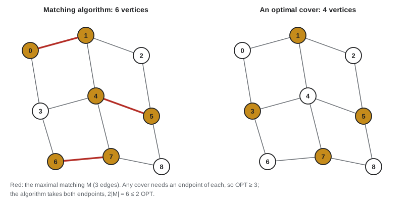
Algorithm. Scan the edges; whenever an edge has neither endpoint in the cover, add both endpoints. Theorem. This is a 2-approximation. Proof. The cover is valid, since every edge is either uncovered when scanned, and then covered, or already covered. The edges that triggered additions form a matching M: no two share an endpoint, because after an edge is taken both its endpoints are in the cover and any later edge touching them is already covered. Any vertex cover, including an optimal one, must contain at least one endpoint of each edge of M, and these endpoints are distinct, so \(\text{OPT} \ge |M|\). The algorithm outputs \(2|M| \le 2\,\text{OPT}\) vertices. The bound is tight: on a complete bipartite graph \(K_{n,n}\) with a perfect matching scanned first, the algorithm takes all 2n vertices while n suffice.

# Two 2-approximations for vertex cover, compared with the exact optimum on random graphs.
import random
from itertools import combinations
random.seed(304)

def matching_cover(E):
    cover = set()
    for u, v in E:                          # scan edges; take both ends of any uncovered edge
        if u not in cover and v not in cover:
            cover |= {u, v}
    return cover

def exact_cover(n, E):
    for k in range(n + 1):
        for C in combinations(range(n), k):
            if all(u in C or v in C for u, v in E): return k

worst, total = 1.0, 0.0
print(" n   edges  optimum  matching cover  ratio")
for trial in range(8):
    n = random.randint(8, 14)
    E = [(u, v) for u, v in combinations(range(n), 2) if random.random() < 0.3]
    random.shuffle(E)
    opt, apx = exact_cover(n, E), len(matching_cover(E))
    worst = max(worst, apx / opt)
    print(f"{n:2d}  {len(E):5d}  {opt:7d}  {apx:14d}  {apx / opt:5.2f}")
print("worst ratio seen:", round(worst, 2), "(the guarantee is 2)")
star = [(0, i) for i in range(1, 9)]
print("on a star with 8 leaves: optimum 1, matching cover", len(matching_cover(star)))

 n   edges  optimum  matching cover  ratio
 9     11        4               6   1.50
 9     19        6               8   1.33
10     13        5               6   1.20
11     11        5               6   1.20
11     16        6               8   1.33
 8      8        3               6   2.00
 9     10        4               6   1.50
 8      9        4               6   1.50
worst ratio seen: 2.0 (the guarantee is 2)
on a star with 8 leaves: optimum 1, matching cover 2

Weighted vertex cover by LP rounding

If vertices have costs \(c_v\), the matching argument fails, but linear programming succeeds. Solve the LP relaxation from lesson 7: minimize \(\sum c_v x_v\) subject to \(x_u + x_v \ge 1\) for each edge and \(0 \le x_v \le 1\). Let \(x^*\) be optimal, and output \(C = \{v : x^*_v \ge 1/2\}\). Every edge has \(x^*_u + x^*_v \ge 1\), so one of the two values is at least \(1/2\), and C is a cover. Its cost is \(\sum_{v \in C} c_v \le \sum_v c_v \cdot 2x^*_v = 2\,\text{LP} \le 2\,\text{OPT}\), because the LP relaxation is a lower bound on the integer optimum. So LP rounding is a 2-approximation for weighted vertex cover. The integrality gap of lesson 7 shows the analysis cannot do better with this LP: on large complete graphs the LP is about n/2 and the optimum is \(n - 1\).

Set cover: the greedy algorithm

Aspen Valley wants to open depots, from a list of candidate sites, so that every delivery zone is within an hour of an open depot, using as few depots as possible. This is SET-COVER: a universe U of n elements (zones) and a family of subsets (the zones each site reaches). The natural greedy algorithm repeatedly picks the set covering the most still-uncovered elements. Theorem. Greedy uses at most \(H(n) \cdot \text{OPT}\) sets, where \(H(n) = 1 + \frac12 + \cdots + \frac1n \le \ln n + 1\). Proof. When greedy picks a set that newly covers t elements, charge each of them \(1/t\); the total charge equals the number of sets chosen. Order the elements in the order they are covered, and consider the k-th last, when at least \(k\) elements remain uncovered. The OPT sets cover those remaining elements, so one of them covers at least \(k/\text{OPT}\) of them, and greedy's choice covers at least as many. So the charge on this element is at most \(\text{OPT}/k\). Summing over k from 1 to n gives at most \(\text{OPT} \cdot H(n)\).

# Greedy set cover: repeatedly take the set covering the most uncovered elements.
# Guarantee: at most H(n) = 1 + 1/2 + ... + 1/n times the optimum.
import random
from itertools import combinations
random.seed(304)

def greedy(U, sets):
    left, chosen = set(U), []
    while left:
        i = max(range(len(sets)), key=lambda j: len(sets[j] & left))
        chosen.append(i); left -= sets[i]
    return chosen

def exact(U, sets):
    for k in range(1, len(sets) + 1):
        for c in combinations(range(len(sets)), k):
            if set().union(*(sets[i] for i in c)) >= U: return k

print(" |U|  sets  optimum  greedy")
for trial in range(6):
    U = set(range(random.randint(12, 20)))
    sets = [set(random.sample(sorted(U), random.randint(2, 6))) for _ in range(12)]
    sets += [{x} for x in U]                       # make sure a cover exists
    print(f"{len(U):4d}  {len(sets):4d}  {exact(U, sets):7d}  {len(greedy(U, sets)):6d}")

# A bad instance for greedy: two disjoint halves cover everything, but greedy takes k sets.
k = 5
A = set(range(0, 2 ** (k + 1) - 2, 2)); B = set(range(1, 2 ** (k + 1) - 1, 2))
U = A | B
blocks, start = [], 0
for i in range(1, k + 1):                          # block i has 2^i elements, half from each side
    size = 2 ** i
    elems = sorted(U)[start:start + size]; start += size
    blocks.append(set(elems))
print("bad instance: optimum 2, greedy uses", len(greedy(U, [A, B] + blocks)), "sets")

 |U|  sets  optimum  greedy
  14    26        5       5
  12    24        3       3
  16    28        5       5
  14    26        5       6
  15    27        5       5
  17    29        6       7
bad instance: optimum 2, greedy uses 5 sets

The logarithmic factor is not an artifact of the proof. Feige showed in 1998 that a ratio of \((1 - \varepsilon) \ln n\) is impossible unless NP problems have slightly superpolynomial algorithms, and Dinur and Steurer in 2014 strengthened this to unless P = NP. So greedy is essentially the best possible polynomial-time algorithm for set cover, a rare case where theory gives a complete answer.

The traveling salesperson problem

General TSP cannot be approximated at all. Suppose some polynomial algorithm guaranteed a tour within a factor \(\alpha\) of optimal. Given a graph G on n vertices, give its edges distance 1 and its non-edges distance \(\alpha n + 1\). If G has a Hamiltonian cycle, the optimum is n, so the algorithm returns a tour of length at most \(\alpha n\), which cannot use any non-edge. If G has none, every tour uses a non-edge and has length more than \(\alpha n\). So the algorithm would decide Hamiltonian cycle, which is NP-complete. Metric TSP, where distances satisfy the triangle inequality \(d(u, w) \le d(u, v) + d(v, w)\), is different, and it is the case that matters for road distances.

The doubling algorithm. Compute a minimum spanning tree T. Deleting one edge of an optimal tour leaves a spanning path, which is a spanning tree, so \(w(T) \le \text{OPT}\). Walk around the tree, traversing each edge twice, for a closed walk of length \(2w(T)\). Then shortcut: skip vertices already visited, going directly to the next new one. By the triangle inequality shortcuts never increase length, so the tour costs at most \(2w(T) \le 2\,\text{OPT}\). Christofides' algorithm (1976; found independently by Serdyukov in the Soviet Union) improves this. The tree has an even number of odd-degree vertices; add a minimum-weight perfect matching M on them, giving a graph with all degrees even, which has an Euler circuit; shortcut it. An optimal tour, shortcut to visit only the odd vertices, splits into two perfect matchings on them, the alternate edges, so \(w(M) \le \text{OPT}/2\), and the tour costs at most \(w(T) + w(M) \le 1.5\,\text{OPT}\).

# Metric TSP on random points: the MST doubling 2-approximation and Christofides' 1.5-approximation,
# compared with the exact optimum from the Held-Karp dynamic program.
import random, math
from functools import lru_cache
random.seed(304)
n = 11
P = [(random.random() * 100, random.random() * 100) for _ in range(n)]
D = [[math.dist(a, b) for b in P] for a in P]

def held_karp():
    @lru_cache(maxsize=None)
    def best(S, j):                                  # shortest path from 0 through set S ending at j
        if S == (1 << j): return D[0][j]
        return min(best(S & ~(1 << j), k) + D[k][j] for k in range(1, n) if S >> k & 1 and k != j)
    full = (1 << n) - 2
    return min(best(full, j) + D[j][0] for j in range(1, n))

def mst():
    inT, parent, key = {0}, [0] * n, [D[0][j] for j in range(n)]
    adj = {v: [] for v in range(n)}
    while len(inT) < n:
        v = min((j for j in range(n) if j not in inT), key=key.__getitem__)
        inT.add(v); adj[v].append(parent[v]); adj[parent[v]].append(v)
        for j in range(n):
            if j not in inT and D[v][j] < key[j]: key[j], parent[j] = D[v][j], v
    return adj

def shortcut(walk):
    seen, tour = set(), []
    for v in walk:
        if v not in seen: seen.add(v); tour.append(v)
    return tour

def length(t): return sum(D[t[i]][t[(i + 1) % len(t)]] for i in range(len(t)))

def double_tree():
    adj, walk = mst(), []
    def dfs(v, p):
        walk.append(v)
        for u in adj[v]:
            if u != p: dfs(u, v); walk.append(v)
    dfs(0, -1)
    return shortcut(walk)

def christofides():
    adj = mst()
    odd = [v for v in range(n) if len(adj[v]) % 2]
    @lru_cache(maxsize=None)
    def pm(mask):                                    # min-weight perfect matching on odd vertices
        if not mask: return 0, ()
        i = (mask & -mask).bit_length() - 1
        best = None
        for j in range(i + 1, n):
            if mask >> j & 1:
                c, m = pm(mask & ~(1 << i) & ~(1 << j))
                if best is None or c + D[i][j] < best[0]: best = (c + D[i][j], m + ((i, j),))
        return best
    multi = {v: list(adj[v]) for v in range(n)}
    for i, j in pm(sum(1 << v for v in odd))[1]: multi[i].append(j); multi[j].append(i)
    stack, walk = [0], []                            # Hierholzer: Euler circuit of tree + matching
    while stack:
        v = stack[-1]
        if multi[v]:
            u = multi[v].pop(); multi[u].remove(v); stack.append(u)
        else: walk.append(stack.pop())
    return shortcut(walk)

opt = held_karp()
mst_w = sum(D[v][u] for v, us in mst().items() for u in us) / 2
for name, t in (("MST doubling", double_tree()), ("Christofides", christofides())):
    print(f"{name:13s} tour {length(t):7.2f}   ratio {length(t) / opt:.3f}")
print(f"optimum       tour {opt:7.2f}   (minimum spanning tree weight {mst_w:.2f})")

MST doubling  tour  422.34   ratio 1.298
Christofides  tour  364.06   ratio 1.119
optimum       tour  325.43   (minimum spanning tree weight 246.59)

For 44 years nobody improved on 1.5 for metric TSP. In 2020 Anna Karlin, Nathan Klein and Shayan Oveis Gharan gave a randomized algorithm with ratio \(1.5 - 10^{-36}\), a tiny improvement that broke a famous barrier, using random spanning trees drawn from a distribution guided by the LP relaxation. For points in the Euclidean plane, Arora and Mitchell independently found polynomial-time approximation schemes in 1996 to 1998: for any fixed \(\varepsilon > 0\), a tour within \(1 + \varepsilon\) of optimal.

Load balancing

Aspen Valley must assign n delivery jobs with durations \(t_j\) to m vans so that the last van finishes as early as possible; the finishing time of the busiest van is the makespan. Graham's list scheduling (1966) assigns each job, in the order given, to the currently least loaded van. Theorem. List scheduling is a \((2 - 1/m)\)-approximation. Proof. Two lower bounds hold: \(\text{OPT} \ge \frac1m \sum_j t_j\), since some van gets at least the average load, and \(\text{OPT} \ge \max_j t_j\). Let van i finish last, and let job j be the last job assigned to it. When j was assigned, van i had the smallest load, which was at most the average of all loads before j, so at most \(\frac1m(\sum t - t_j)\). The makespan is therefore at most \(\frac1m \sum t + (1 - \frac1m) t_j \le \text{OPT} + (1 - \frac1m)\text{OPT}\). Sorting jobs in decreasing order first (longest processing time first) improves the ratio to \(\frac43 - \frac1{3m}\).

# Load balancing on m machines (vans): list scheduling and longest-processing-time-first.
import random
from itertools import product
random.seed(304)

def list_schedule(jobs, m):
    loads = [0] * m
    for t in jobs: loads[loads.index(min(loads))] += t     # next job to the least loaded machine
    return max(loads)

def optimum(jobs, m):
    best = sum(jobs)
    for assign in product(range(m), repeat=len(jobs) - 1):  # job 0 fixed on machine 0 by symmetry
        loads = [0] * m; loads[0] = jobs[0]
        for t, a in zip(jobs[1:], assign): loads[a] += t
        best = min(best, max(loads))
    return best

m = 3
print(" jobs                                list   LPT  optimum")
for trial in range(5):
    jobs = [random.randint(1, 20) for _ in range(9)]
    print(f" {str(jobs):34s} {list_schedule(jobs, m):5d} {list_schedule(sorted(jobs, reverse=True), m):5d} {optimum(jobs, m):8d}")
bad = [1] * (m * (m - 1)) + [m]                              # many small jobs, then one big one
print(f"bad case for list scheduling: list {list_schedule(bad, m)}, optimum {optimum(bad, m)}  (ratio 2 - 1/m = {2 - 1 / m:.2f})")

 jobs                                list   LPT  optimum
 [5, 7, 14, 17, 15, 2, 8, 10, 8]       32    30       29
 [19, 8, 2, 2, 10, 9, 3, 10, 13]       30    27       27
 [5, 6, 13, 15, 19, 12, 20, 7, 10]     40    36       36
 [19, 20, 15, 11, 4, 6, 9, 20, 11]     46    40       39
 [17, 13, 15, 4, 12, 19, 7, 10, 6]     36    35       35
bad case for list scheduling: list 5, optimum 3  (ratio 2 - 1/m = 1.67)

Approximation schemes: knapsack

For some problems the ratio can be pushed as close to 1 as we like. A polynomial-time approximation scheme (PTAS) takes an instance and an \(\varepsilon > 0\) and returns a solution within \(1 + \varepsilon\) of optimal (or at least \((1 - \varepsilon)\) times optimal for maximization) in time polynomial in n for each fixed \(\varepsilon\). It is fully polynomial (FPTAS) if the time is polynomial in both n and \(1/\varepsilon\). Knapsack has an FPTAS built on the value-indexed DP of lesson 3, which runs in \(O(nV)\) time. Let \(v_{\max}\) be the largest value and \(K = \varepsilon v_{\max}/n\). Replace each value by \(\lfloor v_i / K \rfloor\), solve the scaled instance exactly, and return the chosen set. The scaled values are at most \(n/\varepsilon\), so the DP takes \(O(n^3/\varepsilon)\) time.

Theorem. The returned set S has value at least \((1 - \varepsilon)\,\text{OPT}\). Proof. Let \(S^*\) be optimal. Rounding loses less than K per item, so for any set A, \(K \sum_{i \in A} \lfloor v_i/K \rfloor > \sum_{i \in A} v_i - nK\). Since S is optimal for the scaled values, \(\sum_{i \in S} v_i \ge K \sum_{i \in S} \lfloor v_i/K \rfloor \ge K \sum_{i \in S^*} \lfloor v_i/K \rfloor > \text{OPT} - nK = \text{OPT} - \varepsilon v_{\max}\). Since any single item fits (discard those that do not), \(\text{OPT} \ge v_{\max}\), so the value is at least \((1 - \varepsilon)\,\text{OPT}\).

# A fully polynomial-time approximation scheme for knapsack: scale values down by
# K = eps * vmax / n, round down, solve the scaled instance exactly with the value-indexed DP.
import random
random.seed(304)
n = 40
items = [(random.randint(10, 60), random.choice([random.randint(100, 999), random.randint(10 ** 4, 10 ** 5)]))
         for _ in range(n)]                                   # (weight, value): values of mixed sizes
W = 400

def exact_by_weight():                                        # O(nW): fine because W is small here
    K = [0] * (W + 1)
    for w, v in items:
        for c in range(W, w - 1, -1): K[c] = max(K[c], K[c - w] + v)
    return K[W]

def solve_scaled(eps):
    vmax = max(v for _, v in items)
    Kf = eps * vmax / n
    vals = [int(v // Kf) for _, v in items]
    V = sum(vals); INF = float("inf")
    M = [[0] + [INF] * V]                                     # M[i][t]: first i items, scaled value t
    for (w, _), v in zip(items, vals):
        prev = M[-1]; cur = prev[:]
        for t in range(v, V + 1):
            if prev[t - v] + w < cur[t]: cur[t] = prev[t - v] + w
        M.append(cur)
    t = max(t for t in range(V + 1) if M[n][t] <= W)
    S = []
    for i in range(n, 0, -1):                                 # recover the chosen set
        if M[i][t] != M[i - 1][t]:
            S.append(i - 1); t -= vals[i - 1]
    return sum(items[i][1] for i in S), n * (V + 1)

opt = exact_by_weight()
print("exact optimum", opt)
for eps in (0.9, 0.5, 0.25, 0.1):
    val, work = solve_scaled(eps)
    print(f"eps = {eps:4}: value {val}  ratio {val / opt:.4f}  (guarantee >= {1 - eps:.2f})  table cells {work:,}")

exact optimum 929552
eps =  0.9: value 929552  ratio 1.0000  (guarantee >= 0.10)  table cells 19,520
eps =  0.5: value 929552  ratio 1.0000  (guarantee >= 0.50)  table cells 35,280
eps = 0.25: value 929552  ratio 1.0000  (guarantee >= 0.75)  table cells 71,040
eps =  0.1: value 929552  ratio 1.0000  (guarantee >= 0.90)  table cells 178,800

Limits of approximation

Problems differ sharply in how well they can be approximated. Knapsack has an FPTAS; Euclidean TSP has a PTAS but, being strongly NP-hard, no FPTAS unless P = NP; vertex cover has a 2-approximation; set cover has \(\ln n\); general TSP has no constant ratio at all. Lower bounds come from the PCP theorem (Arora and Safra; Arora, Lund, Motwani, Sudan and Szegedy; 1992), which says that every NP statement has a proof that can be checked, with high confidence, by reading only a constant number of randomly chosen bits. Equivalently, it is NP-hard to tell satisfiable 3SAT formulas from those where every assignment violates a constant fraction of clauses. Building on it, Håstad proved in 2001 that a random assignment's ratio of \(7/8\) for MAX-3SAT is optimal unless P = NP. For vertex cover, Dinur and Safra proved that a ratio below 1.36 is NP-hard, and Khot and Regev showed in 2008 that beating 2 by any constant would refute Khot's Unique Games Conjecture.

Worked examples