Capstone: coping with hardness — parameterized, exact exponential and heuristic algorithms

It is Saturday at Aspen Valley Couriers. Sixty stops must be visited by a few vans, each with a weight limit and a shift length, with some customers requiring delivery windows. This vehicle routing problem contains the traveling salesperson problem, knapsack and scheduling as special cases, so it is NP-hard several times over. Lesson 10 offered approximation algorithms with guarantees. This final lesson completes the toolkit with three other responses to hardness: exact exponential algorithms that are much faster than brute force, parameterized algorithms that are exponential only in some small quantity, and heuristics that have no worst-case guarantee but work extremely well in practice, especially when combined with lower bounds that measure how good their answers are. It ends by drawing the whole course together into a method for facing a new problem.

Exact exponential algorithms

If an instance must be solved exactly and it is not too large, the goal is to make the exponential as small as possible. The difference matters enormously: an \(O(2^n)\) algorithm handles twice the n of an \(O(4^n)\) one in the same time. Held–Karp for TSP. Bellman, and independently Held and Karp, gave in 1962 a dynamic program over subsets. Let \(\text{best}(S, j)\) be the length of a shortest path that starts at city 0, visits exactly the cities in S and ends at \(j \in S\). Then \(\text{best}(S, j) = \min_{k \in S \setminus \{j\}} (\text{best}(S \setminus \{j\}, k) + d(k, j))\), and the optimal tour is \(\min_j (\text{best}(V, j) + d(j, 0))\). There are \(2^n n\) states, each taking \(O(n)\) time, for \(O(2^n n^2)\) total, against \((n-1)!/2\) tours for brute force. More than sixty years later this is still the best known worst-case bound for general TSP.

# Held-Karp dynamic programming for TSP: O(2^n n^2) instead of (n-1)! tours.
# best[S][j] = shortest path that starts at 0, visits exactly the set S, and ends at j.
import random, math
from itertools import permutations
random.seed(304)

def held_karp(D):
    n = len(D); FULL = 1 << n
    best = [[math.inf] * n for _ in range(FULL)]
    best[1][0] = 0
    steps = 0
    for S in range(1, FULL, 2):                      # every set containing vertex 0
        for j in range(n):
            if not S >> j & 1 or best[S][j] == math.inf: continue
            for k in range(n):
                if S >> k & 1: continue
                steps += 1
                T = S | 1 << k
                if best[S][j] + D[j][k] < best[T][k]: best[T][k] = best[S][j] + D[j][k]
    return min(best[FULL - 1][j] + D[j][0] for j in range(1, n)), steps

def brute(D):
    n = len(D)
    return min(sum(D[t[i]][t[i + 1]] for i in range(n - 1)) + D[t[-1]][0]
               for t in ((0,) + p for p in permutations(range(1, n)))), math.factorial(n - 1)

print(" n   Held-Karp steps   brute-force tours   same answer")
for n in (6, 8, 10):
    P = [(random.random(), random.random()) for _ in range(n)]
    D = [[math.dist(a, b) for b in P] for a in P]
    (h, hs), (b, bs) = held_karp(D), brute(D)
    print(f"{n:2d}   {hs:15,d}   {bs:17,d}   {abs(h - b) < 1e-9}")
for n in (20, 30):
    print(f"{n:2d}   about {2 ** n * n * n:.1e} steps   {math.factorial(n - 1):.1e} tours")

 n   Held-Karp steps   brute-force tours   same answer
 6               165                 120   True
 8             1,351               5,040   True
10             9,225             362,880   True
20   about 4.2e+08 steps   1.2e+17 tours
30   about 9.7e+11 steps   8.8e+30 tours

Meet in the middle. For subset sum with n numbers, brute force checks \(2^n\) subsets. Horowitz and Sahni (1974) split the numbers into two halves, list the \(2^{n/2}\) subset sums of each half, sort one list, and for each sum s of the other half search for \(T - s\). That takes \(O(2^{n/2} n)\) time, the square root of brute force, at the cost of \(O(2^{n/2})\) memory. The same idea speeds up attacks on block ciphers and some lattice problems. Branch and bound explores a search tree of partial solutions but prunes any branch whose optimistic bound, often from an LP relaxation or a minimum spanning tree, cannot beat the best solution found so far. It has no better worst case than brute force, but good bounds prune most of the tree on real instances; it is the core of every integer programming solver.

# Meet in the middle for SUBSET-SUM (Horowitz and Sahni, 1974): split the numbers in half,
# list all 2^(n/2) sums of each half, sort one list, and binary-search for complements.
import random, bisect
from itertools import combinations
random.seed(304)

def sums(nums):
    out = [0]
    for x in nums: out += [s + x for s in out]
    return out

def mitm(nums, T):
    L, R = sums(nums[:len(nums) // 2]), sorted(sums(nums[len(nums) // 2:]))
    for s in L:
        i = bisect.bisect_left(R, T - s)
        if i < len(R) and R[i] == T - s: return True, len(L) + len(R)
    return False, len(L) + len(R)

print(" n   answer   meet-in-the-middle list sizes   2^n subsets")
for n in (16, 24, 32):
    nums = [random.randint(10 ** 8, 10 ** 9) for _ in range(n)]
    T = sum(random.sample(nums, n // 3)) + 1          # usually not reachable: a hard case
    ans, work = mitm(nums, T)
    print(f"{n:2d}   {ans!s:6s}   {work:29,d}   {2 ** n:11,d}")

 n   answer   meet-in-the-middle list sizes   2^n subsets
16   False                              512        65,536
24   False                            8,192    16,777,216
32   False                          131,072   4,294,967,296

How small can the exponential get? The Exponential Time Hypothesis (Impagliazzo and Paturi, 2001) conjectures that 3SAT cannot be solved in time \(2^{o(n)}\), and its strong form, SETH, that CNF-SAT cannot be solved in time \(O(2^{(1-\varepsilon)n})\) for any \(\varepsilon > 0\). Like \(\text{P} \ne \text{NP}\), these are unproved, but they give a fine-grained theory: under ETH, many classic algorithms, such as the \(2^{O(\sqrt n)}\) algorithms for planar graph problems, are essentially optimal.

Parameterized algorithms

Often the hard part of a problem is controlled by a small number. Aspen Valley may want at most \(k = 12\) inspectors to cover all streets of a large network: vertex cover with a small k. Trying all \(\binom{n}{k}\) sets is hopeless for \(n = 400\), but an algorithm with running time \(f(k) \cdot n^{O(1)}\), where f may be exponential but the polynomial does not depend on k, is practical. Problems with such algorithms are fixed-parameter tractable (FPT), a theory developed by Downey and Fellows in the 1990s.

A bounded search tree for vertex cover. Take any edge \((u, v)\). Every vertex cover contains u or v, so try both: put u in the cover and recurse on the graph without u with budget \(k - 1\), and if that fails, do the same with v. The recursion depth is at most k and each node branches twice, so the tree has at most \(2^{k+1}\) nodes, each taking \(O(m)\) time: \(O(2^k m)\) overall. A kernel. Buss observed that a vertex of degree greater than k must be in every cover of size at most k, since otherwise all its more than k neighbors would be needed. Put such vertices in the cover, lowering k. Afterwards every vertex has degree at most k, so a cover of size k touches at most \(k^2\) edges; if more remain, answer no. What is left is a kernel of at most \(k^2\) edges, whose size depends only on k. Refined branching rules reduced the base: Chen, Kanj and Xia gave an \(O(1.2738^k + kn)\) algorithm in 2010.

# Fixed-parameter algorithms for VERTEX-COVER with parameter k.
# Bounded search tree: some endpoint of any edge (u, v) is in every cover, so branch on u or v.
# Depth at most k, so at most 2^k leaves: O(2^k m) time. Buss kernel: a vertex of degree > k
# must be in any cover of size <= k; afterwards more than k^2 edges means "no".
import random
from math import comb
random.seed(304)

def vc_branch(E, k, stats):
    stats[0] += 1
    if not E: return set()
    if k == 0: return None
    u, v = E[0]
    for w in (u, v):
        rest = [e for e in E if w not in e]
        S = vc_branch(rest, k - 1, stats)
        if S is not None: return S | {w}
    return None

def kernel(E, k):
    forced = set()
    while True:
        deg = {}
        for u, v in E: deg[u] = deg.get(u, 0) + 1; deg[v] = deg.get(v, 0) + 1
        high = [x for x, d in deg.items() if d > k - len(forced)]
        if not high: break
        forced.add(high[0]); E = [e for e in E if high[0] not in e]
    return E, k - len(forced), forced

n = 400                                           # a large sparse graph with a planted cover of size 12
cover = random.sample(range(n), 12)
E = list({(min(c, x), max(c, x)) for c in cover for x in random.sample(range(n), 6) if x != c})
E += [(cover[0], x) for x in random.sample(range(n), 40) if x != cover[0]]    # one hub
E = sorted(set(E))
for k in (10, 11, 12):
    Ek, kk, forced = kernel(E, k)
    stats = [0]
    S = None if kk < 0 or len(Ek) > kk * kk else vc_branch(Ek, kk, stats)
    found = (S | forced) if S is not None else None
    print(f"k = {k}: kernel keeps {len(Ek)} edges, k' = {kk};  search nodes {stats[0]:5d};  "
          f"cover {'found, size ' + str(len(found)) if found else 'none'}")
print(f"brute force would test C({n}, 12) = {comb(n, 12):.2e} vertex sets")

k = 10: kernel keeps 66 edges, k' = 9;  search nodes  1023;  cover none
k = 11: kernel keeps 66 edges, k' = 10;  search nodes  2047;  cover none
k = 12: kernel keeps 66 edges, k' = 11;  search nodes  3968;  cover found, size 12
brute force would test C(400, 12) = 2.97e+22 vertex sets

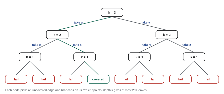
Not every parameter helps. Clique parameterized by its size k is believed not to be FPT: it is complete for the class W[1], and no \(f(k) n^{O(1)}\) algorithm is expected. Other useful parameters include the treewidth of a graph, which lets the tree DP of lesson 3 extend to many NP-hard problems in time \(2^{O(w)} n\) for width w (Courcelle's theorem makes this sweeping for problems expressible in a certain logic), and the number of distinct numbers or the solution size in scheduling problems. Choosing a parameter that is small in your instances is a modeling decision as much as an algorithmic one.

Heuristics and local search

For the Saturday routes, the dispatcher needs a good answer in seconds for 60 stops, and nobody needs a proof of optimality. Construction heuristics build a solution greedily, such as nearest neighbor: from the current stop go to the closest unvisited one. Local search then improves it with small changes. The 2-opt move for TSP removes two edges of the tour and reconnects the two paths the other way, which reverses a segment; it is applied whenever it shortens the tour, until no improving move exists. The result is a local optimum: no single 2-opt move helps, though the tour need not be globally optimal. Without crossing edges, which a 2-opt move always removes in the plane, tours on random instances are usually only about 5% longer than optimal.

# Heuristics for a 60-stop route: greedy closest-stop tour, then 2-opt local search
# (reverse a segment whenever that shortens the tour). The MST weight is a lower bound on OPT.
import random, math
random.seed(304)
n = 60
P = [(random.random() * 50, random.random() * 50) for _ in range(n)]       # stops in a 50 km square
D = [[math.dist(a, b) for b in P] for a in P]
length = lambda t: sum(D[t[i]][t[(i + 1) % n]] for i in range(n))

tour, left = [0], set(range(1, n))
while left:                                        # closest unvisited stop each time
    nxt = min(left, key=lambda j: D[tour[-1]][j]); tour.append(nxt); left.remove(nxt)
nn = length(tour)

improved, passes = True, 0
while improved:                                    # 2-opt until no improving move exists
    improved = False; passes += 1
    for i in range(n - 1):
        for j in range(i + 2, n if i else n - 1):
            a, b, c, d = tour[i], tour[i + 1], tour[j], tour[(j + 1) % n]
            if D[a][c] + D[b][d] < D[a][b] + D[c][d] - 1e-12:
                tour[i + 1:j + 1] = reversed(tour[i + 1:j + 1]); improved = True

key, inT, mst = [D[0][j] for j in range(n)], {0}, 0.0
while len(inT) < n:                                # Prim's algorithm for the lower bound
    v = min((j for j in range(n) if j not in inT), key=key.__getitem__)
    mst += key[v]; inT.add(v)
    for j in range(n):
        if j not in inT: key[j] = min(key[j], D[v][j])
print(f"closest-stop tour:       {nn:6.1f} km")
print(f"after 2-opt ({passes} passes): {length(tour):6.1f} km")
print(f"MST lower bound:         {mst:6.1f} km  -> 2-opt tour is within {length(tour) / mst:.2f} of the bound")

closest-stop tour:        364.3 km
after 2-opt (4 passes):  321.6 km
MST lower bound:          248.3 km  -> 2-opt tour is within 1.30 of the bound

Local search can get stuck in poor local optima. Simulated annealing (Kirkpatrick, Gelatt and Vecchi, 1983) sometimes accepts worsening moves, with a probability that decreases over time, to escape them. Tabu search, genetic algorithms and large neighborhood search are other metaheuristics. The Lin–Kernighan heuristic (1973) and its modern implementation LKH find tours within a fraction of a percentage point of optimal for instances with millions of cities. Pair a heuristic with a lower bound, such as an MST, a 1-tree, or an LP relaxation, and you get a quality certificate: the program above shows its 2-opt tour is within a known factor of the bound, so within that factor of the optimum.

Solvers: using the hardness of others

Often the best way to solve an NP-hard problem is to reduce it to one that specialists have spent decades engineering. Modern SAT solvers use conflict-driven clause learning (CDCL), which analyses each dead end to learn a new clause that prevents similar failures, together with clever branching heuristics and restarts; they routinely solve industrial formulas with millions of variables from hardware verification and software testing. Integer programming solvers combine LP relaxations, branch and bound and cutting planes. The Concorde TSP solver, built on LP-based branch and cut by Applegate, Bixby, Chvátal and Cook, proved an optimal tour for an 85,900-city instance from a chip layout in 2006. Reducing your problem to SAT or ILP, the reverse of the reductions in lesson 9, is a powerful practical technique, since solver improvements then come for free.

The course in one view

The guide is not a flowchart to apply mechanically, but it captures the habits this course has tried to build. Ask first whether the problem is secretly one you know how to solve efficiently; most problems that look new are not. If you cannot find an efficient algorithm after honest effort, look for a reduction that proves hardness, so that you can stop searching for the impossible with a clear conscience. Then decide which demand to relax, exactness, worst-case speed, generality or certainty, according to what the users of the answer actually need. And whatever you build, test it against brute force on small inputs and compute lower bounds on large ones, so that you know how good it really is.

For Aspen Valley the answer is a combination. Parcels are assigned to vans with a knapsack-style DP when weights are small; drivers are matched to vans by flow; each van's route starts from a construction heuristic, is improved by 2-opt and Or-opt moves, and is checked against an LP bound; and the weekly depot plan, a set cover with a few dozen sites, is solved exactly by an integer programming solver overnight. Each piece uses the right tool for its size and its demands, which is what algorithm design in practice looks like. CMPUT-474 continues the story on the theoretical side, and courses on optimization, machine learning and operations research build on the methods here.

Worked examples