Randomized algorithms: Las Vegas, Monte Carlo and hashing

A randomized algorithm makes random choices as it runs. That sounds like a weakness, but randomness is one of the most practical tools in algorithm design. Random choices defeat worst-case inputs, because no fixed input can be bad for most of the algorithm's choices; they make algorithms simpler; and they make some problems, such as verifying a matrix product or finding a minimum cut, dramatically faster. The guarantees are about the algorithm's own coins, not about the input: for every input, the expected running time is small, or the probability of a wrong answer is small. This lesson develops the two kinds of randomized algorithm and the probabilistic tools needed to analyze them.

Las Vegas and Monte Carlo

A Las Vegas algorithm always returns a correct answer, but its running time is a random variable; we bound its expected running time for every input. Randomized quicksort is the classic example. A Monte Carlo algorithm always runs within a fixed time bound, but its answer may be wrong with some small probability. Miller–Rabin primality testing is the classic example: it may declare a composite number prime, but with probability at most \(4^{-k}\) after k independent rounds. The two kinds convert partly into each other. A Las Vegas algorithm stopped after twice its expected time fails with probability at most 1/2 by Markov's inequality, giving a Monte Carlo algorithm. A Monte Carlo algorithm whose answers can be checked quickly can be rerun until a check succeeds, giving a Las Vegas algorithm.

Monte Carlo errors can be amplified away. If an algorithm with one-sided error never errs on no-instances and says yes on yes-instances with probability at least p, running it k times independently and saying yes if any run does fails with probability at most \((1 - p)^k \le e^{-pk}\). For two-sided error at most 1/3, take the majority of k runs; a Chernoff bound shows the error falls exponentially in k. In practice, 50 rounds bring the error probability below the chance of a hardware fault during the computation.

Tools: linearity of expectation and indicators

Most analyses rest on one fact: the expectation of a sum is the sum of the expectations, \(E[X + Y] = E[X] + E[Y]\), whether or not X and Y are independent. The standard technique writes a complicated quantity as a sum of indicator random variables, each 1 if some event happens and 0 otherwise, so that its expectation is a sum of probabilities. Randomized quicksort. Let \(z_1 < z_2 < \cdots < z_n\) be the sorted keys and \(X_{ij}\) the indicator that \(z_i\) and \(z_j\) are ever compared. They are compared exactly when the first pivot chosen from \(\{z_i, \dots, z_j\}\) is one of the two, because a pivot strictly between them separates them forever, and any pivot outside this range leaves them together. Each of the \(j - i + 1\) values is equally likely to be first, so \(\Pr[X_{ij} = 1] = 2/(j - i + 1)\). Hence the expected number of comparisons is \(\sum_{i < j} \frac{2}{j - i + 1} \le 2n H_n \approx 2n \ln n\), which CMPUT-204 computed exactly. This bound holds for every input.

Randomized quickselect finds the k-th smallest element by partitioning around a random pivot and recursing into one side only. Call a pivot good if it lands in the middle half of the current array; then the side kept has at most 3/4 of the elements. A good pivot appears with probability 1/2, so on average two rounds pass between successive shrinkings by a factor 3/4. The expected total work is at most \(2(n + \frac34 n + (\frac34)^2 n + \cdots) = 8n\), linear. The median-of-medians algorithm of CMPUT-204 achieves linear time deterministically, but with a larger constant and more code.

# Randomized quicksort and quickselect: count comparisons and compare with the expectations.
import random, math
random.seed(304)

def quicksort(a, count):
    if len(a) <= 1: return a
    p = random.choice(a)
    less, equal, more = [], [], []
    for x in a:
        count[0] += 1
        (less if x < p else more if x > p else equal).append(x)
    return quicksort(less, count) + equal + quicksort(more, count)

def quickselect(a, k, count):           # k-th smallest, 0-based
    while True:
        p = random.choice(a)
        less = [x for x in a if x < p]; equal = [x for x in a if x == p]
        count[0] += len(a)
        if k < len(less): a = less
        elif k < len(less) + len(equal): return p
        else: k -= len(less) + len(equal); a = [x for x in a if x > p]

print("     n   quicksort comparisons   2n ln n    quickselect (median) comparisons / n")
for n in (1000, 10000, 100000):
    a = random.sample(range(10 * n), n)
    c = [0]; s = quicksort(a, c); assert s == sorted(a)
    q = [0]; m = quickselect(a, n // 2, q); assert m == s[n // 2]
    print(f"{n:6d}   {c[0]:21d}   {2 * n * math.log(n):9.0f}    {q[0] / n:6.2f}")

     n   quicksort comparisons   2n ln n    quickselect (median) comparisons / n
  1000                   12136       13816      2.55
 10000                  155915      184207      4.74
100000                 2116030     2302585      3.40

Universal hashing

A hash table with chaining stores n keys in m slots, using a hash function h to choose a slot. If h spreads the keys evenly, operations take \(O(1 + n/m)\) expected time. But any fixed h has bad inputs: for \(h(x) = x \bmod m\), every multiple of m lands in slot 0, and an attacker who knows h can send exactly such keys, a real denial-of-service technique against web servers. Carter and Wegman's answer (1979) is to pick h at random from a family designed so that every pair of keys rarely collides. A family H of functions from keys to \(\{0, \dots, m - 1\}\) is universal if for every pair of distinct keys \(x \ne y\), \(\Pr_{h \in H}[h(x) = h(y)] \le 1/m\).

Theorem. With h drawn from a universal family, the expected number of other keys in the slot of any key x is at most \(n/m\). Proof. For each other key y let \(C_y\) indicate \(h(x) = h(y)\). The expected chain length is \(\sum_y E[C_y] = \sum_y \Pr[h(x) = h(y)] \le n/m\) by linearity. A universal family. Choose a prime \(p\) larger than every key and let \(h_{ab}(x) = ((ax + b) \bmod p) \bmod m\) for \(1 \le a < p\) and \(0 \le b < p\). For distinct x and y, the map from \((a, b)\) to \((ax + b \bmod p,\ ay + b \bmod p)\) is a bijection onto pairs of distinct residues, because the system can be solved for a and b given the two residues. So the pair of residues is uniformly random among distinct pairs, and the fraction of those pairs that agree modulo m is at most \(1/m\).

# Universal hashing defeats adversarial keys. A fixed hash h(x) = x mod m sends all multiples
# of m to slot 0; a random member of h_ab(x) = ((a x + b) mod p) mod m spreads them out.
import random
random.seed(304)
m, p = 101, 1_000_003                       # table size and a prime larger than every key
keys = [m * i for i in range(1, 2001)]      # an unlucky (or malicious) set of keys

def longest_chain(h):
    slots = [0] * m
    for k in keys: slots[h(k)] += 1
    return max(slots), sum(c * (c - 1) // 2 for c in slots)

print("fixed hash x mod m:      longest chain %d, colliding pairs %d" % longest_chain(lambda x: x % m))
for trial in range(3):
    a, b = random.randrange(1, p), random.randrange(p)
    print("random h_ab, trial %d:   longest chain %d, colliding pairs %d" % ((trial + 1,) + longest_chain(lambda x: (a * x + b) % p % m)))
n = len(keys)
print("expected colliding pairs for a universal family: at most n(n-1)/(2m) =", n * (n - 1) // (2 * m))

fixed hash x mod m:      longest chain 2000, colliding pairs 1999000
random h_ab, trial 1:   longest chain 23, colliding pairs 18985
random h_ab, trial 2:   longest chain 21, colliding pairs 18824
random h_ab, trial 3:   longest chain 21, colliding pairs 18830
expected colliding pairs for a universal family: at most n(n-1)/(2m) = 19792

Universal hashing guarantees expected behavior for every set of keys, chosen before the random function. Stronger properties give stronger guarantees: perfect hashing (Fredman, Komlós and Szemerédi, 1984) builds a two-level table with no collisions at all for a static set, using linear space; cuckoo hashing (Pagh and Rodler, 2001) gives worst-case constant lookup time. Python's own dictionaries randomize string hashing by default for exactly the security reason above.

Verifying a matrix product

Suppose a library returns C as the product of two \(n \times n\) matrices A and B. Checking it by recomputing AB costs as much as computing it. Freivalds' algorithm (1977) picks a random vector r with independent entries 0 or 1 and checks whether \(A(Br) = Cr\), which takes three matrix–vector products, \(O(n^2)\) time. If \(AB = C\) the check always passes. If not, let \(D = AB - C \ne 0\), with some nonzero entry \(d_{ij}\). Then \((Dr)_i = d_{ij} r_j + s\), where s does not depend on \(r_j\). Whatever s is, at most one of the two values of \(r_j\) makes this zero, so the check fails with probability at least 1/2. After k independent trials a wrong product survives with probability at most \(2^{-k}\). This is a Monte Carlo algorithm with one-sided error, and no deterministic \(O(n^2)\) verifier is known.

# Freivalds' check (1977): is A B = C?  Pick random 0/1 vector r and compare A(Br) with Cr.
# O(n^2) per trial; if AB != C each trial catches it with probability at least 1/2.
import random
random.seed(304)
n = 60
A = [[random.randint(0, 9) for _ in range(n)] for _ in range(n)]
B = [[random.randint(0, 9) for _ in range(n)] for _ in range(n)]
C = [[sum(A[i][k] * B[k][j] for k in range(n)) for j in range(n)] for i in range(n)]
bad = [row[:] for row in C]; bad[17][42] += 1               # one wrong entry

def mv(M, v): return [sum(x * y for x, y in zip(row, v)) for row in M]
def trial(A, B, C):
    r = [random.randint(0, 1) for _ in range(n)]
    return mv(A, mv(B, r)) == mv(C, r)

print("correct product passes 20 of 20 trials:", all(trial(A, B, C) for _ in range(20)))
caught = sum(not trial(A, B, bad) for _ in range(1000))
print(f"wrong product caught in {caught} of 1000 single trials (at least about half expected)")
print("probability 20 trials all miss an error: at most", 0.5 ** 20)
print("work per trial ~", 3 * n * n, "multiplications, versus", n ** 3, "to recompute AB")

correct product passes 20 of 20 trials: True
wrong product caught in 512 of 1000 single trials (at least about half expected)
probability 20 trials all miss an error: at most 9.5367431640625e-07
work per trial ~ 10800 multiplications, versus 216000 to recompute AB

Karger's minimum cut algorithm

The global minimum cut of an undirected graph is a smallest set of edges whose removal disconnects it. It can be found with \(n - 1\) maximum flow computations, but David Karger's 1993 algorithm is strikingly simpler. Random contraction: while more than two vertices remain, pick a uniformly random edge and contract it, merging its endpoints into one vertex and keeping parallel edges but deleting self-loops. When two vertices remain, the edges between them form a cut. Theorem. A fixed minimum cut C, of size k, survives with probability at least \(2/(n(n-1))\). Proof. Every vertex has degree at least k, since its edges form a cut, so a graph with i vertices has at least \(ik/2\) edges. The cut survives a step exactly when the chosen edge is not in C, which has probability at least \(1 - k/(ik/2) = 1 - 2/i\). Multiplying over \(i = n, n - 1, \dots, 3\) gives \(\prod_{i=3}^{n} \frac{i - 2}{i} = \frac{2}{n(n - 1)}\), a telescoping product.

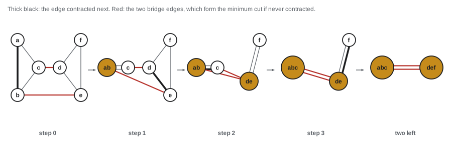
One run is likely to fail, but repeating it \(\binom{n}{2} \ln(1/\delta)\) times and keeping the smallest cut found fails with probability at most \((1 - 1/\binom{n}{2})^{\binom{n}{2}\ln(1/\delta)} \le \delta\). The analysis has a pleasing corollary: since each minimum cut survives with probability at least \(1/\binom{n}{2}\) and these events are disjoint, a graph has at most \(\binom{n}{2}\) minimum cuts. Karger and Stein (1996) sped the algorithm up by contracting only down to about \(n/\sqrt2\) vertices before branching, reaching \(O(n^2 \log^3 n)\) time.

# Karger's random contraction for minimum cut. One run succeeds with probability >= 2/(n(n-1));
# repeating about n^2 ln n times makes failure very unlikely.
import random, math
random.seed(304)

def contract(n, edges):
    leader = list(range(n))
    def find(x):
        while leader[x] != x: leader[x] = leader[leader[x]]; x = leader[x]
        return x
    groups, order = n, edges[:]
    random.shuffle(order)                     # contracting edges in random order = Kruskal on random weights
    for u, v in order:
        if groups == 2: break
        a, b = find(u), find(v)
        if a != b: leader[a] = b; groups -= 1
    return sum(1 for u, v in edges if find(u) != find(v))

# Two dense clusters of 6 vertices joined by 2 edges: the minimum cut is 2.
n = 12
edges = [(u, v) for c in (range(0, 6), range(6, 12)) for u in c for v in c if u < v]
edges += [(0, 6), (3, 9)]
runs = 2000
hits = sum(contract(n, edges) == 2 for _ in range(runs))
print(f"single run finds the minimum cut in {hits} of {runs} runs ({hits / runs:.3f});"
      f" the bound is {2 / (n * (n - 1)):.3f}")
reps = int(n * (n - 1) / 2 * math.log(100))
print(f"repeating {reps} times fails with probability at most {(1 - 2 / (n * (n - 1))) ** reps:.4f}")
print("best of 50 runs:", min(contract(n, edges) for _ in range(50)))

single run finds the minimum cut in 630 of 2000 runs (0.315); the bound is 0.015
repeating 303 times fails with probability at most 0.0098
best of 50 runs: 2

Primality testing

Fermat's little theorem says that if n is prime then \(a^{n-1} \equiv 1 \pmod n\) for every a coprime to n. Testing this for random a catches most composites, but Carmichael numbers, the smallest being \(561 = 3 \cdot 11 \cdot 17\), satisfy it for every coprime a. The Miller–Rabin test (Miller 1976, Rabin 1980) adds a second check: write \(n - 1 = 2^s d\) with d odd, and look at \(a^d, a^{2d}, \dots, a^{2^s d}\). For a prime, this sequence is all 1s or reaches \(-1\) before it reaches 1, because 1 has only the square roots 1 and \(-1\) modulo a prime. For an odd composite, at least three quarters of the bases violate this, so each random base exposes a composite with probability at least 3/4. Since 2002 the AKS algorithm shows primality is in P deterministically, but Miller–Rabin remains the method used in practice, for example to generate RSA keys, and CMPUT-474 places it in the class of problems with efficient randomized algorithms.

# Miller-Rabin: a Monte Carlo test with one-sided error. Fermat's test is fooled by
# Carmichael numbers such as 561 = 3 * 11 * 17; Miller-Rabin is not.
import random
random.seed(304)

def fermat(n, a): return pow(a, n - 1, n) == 1
def miller_rabin(n, a):
    d, s = n - 1, 0
    while d % 2 == 0: d //= 2; s += 1
    x = pow(a, d, n)
    if x in (1, n - 1): return True
    for _ in range(s - 1):
        x = x * x % n
        if x == n - 1: return True
    return False                                  # a is a witness: n is certainly composite

for n in (561, 1105, 1729, 2 ** 61 - 1):
    bases = [a for a in range(2, 200) if __import__("math").gcd(a, n) == 1]
    f = sum(fermat(n, a) for a in bases); m = sum(miller_rabin(n, a) for a in bases)
    print(f"n = {n}: coprime bases fooling Fermat {f}/{len(bases)}, fooling Miller-Rabin {m}/{len(bases)}")

n = 561: coprime bases fooling Fermat 113/113, fooling Miller-Rabin 3/113
n = 1105: coprime bases fooling Fermat 138/138, fooling Miller-Rabin 5/138
n = 1729: coprime bases fooling Fermat 148/148, fooling Miller-Rabin 23/148
n = 2305843009213693951: coprime bases fooling Fermat 198/198, fooling Miller-Rabin 198/198

When to reach for randomness

Randomness helps most when a worst case comes from an unlucky interaction between input and algorithm (pivots, hash functions), when checking is much easier than computing (Freivalds, primality), and when a simple random process has a provable chance of success (contraction, random assignment). Whether randomness is ever necessary for efficient algorithms is a deep open question: most researchers believe that every problem solvable in randomized polynomial time is solvable deterministically, and Impagliazzo and Wigderson showed in 1997 that this follows from plausible circuit lower bounds. In practice, random bits come from pseudorandom generators, and the analyses here hold provided the generator is good enough for the purpose.

Worked examples