Traffic flow fundamentals

On a winter morning after a heavy snowfall, a plow from the operations center heads north on the two-lane highway beyond the city at a steady, slow speed. Within minutes a line of cars builds up behind it, and the line grows longer for as long as the plow stays on the road. Drivers in the line experience it as a nuisance; traffic engineers see it as a textbook example of a shockwave, a moving boundary between two traffic states. To understand it, and to analyze the capacity of roads in later lessons, we need the basic variables of traffic flow and the relationships between them.

Flow, speed and density

Three variables describe a traffic stream at the macroscopic level. Flow (or volume) \(q\) is the number of vehicles passing a point per unit time, usually expressed in vehicles per hour. Density (or concentration) \(k\) is the number of vehicles occupying a length of road at an instant, in vehicles per kilometer or per mile, usually per lane. Speed \(v\) is the rate of motion of the vehicles. These are linked by the fundamental relationship

which follows from counting: if vehicles at density \(k\) move at speed \(v\), then in one hour a stretch of road \(v\) long passes the observer, containing \(kv\) vehicles. The relationship holds exactly only when speed is the space-mean speed, described below.

At the microscopic level, the same stream is described by the spacing and timing of individual vehicles. Headway \(h\) is the time between successive vehicles passing a point, and spacing \(s\) is the distance between them. The averages are reciprocals of the macroscopic variables: mean headway is \(1/q\) and mean spacing is \(1/k\). A flow of 1,800 vehicles per hour per lane corresponds to an average headway of 2 seconds, and a density of 25 vehicles per kilometer per lane corresponds to an average spacing of 40 m.

Two kinds of average speed

There are two ways to average the speeds of vehicles. The time-mean speed is the arithmetic mean of the speeds of vehicles passing a point over a period, which is what a radar gun or a loop detector measures. The space-mean speed is the mean speed of the vehicles occupying a length of road at an instant, or equivalently the length of the road divided by the average travel time across it. Because faster vehicles pass a point more often than slower ones, the time-mean speed is always at least as large as the space-mean speed. The space-mean speed is the harmonic mean of the spot speeds:

For example, if two vehicles pass a detector at 30 and 60 mph, the time-mean speed is 45 mph, but the space-mean speed is \(2/(1/30 + 1/60) = 40\) mph. The space-mean speed is the one to use in \(q = kv\) and in travel time calculations.

The Greenshields model

How does speed change as density rises? When the road is nearly empty, drivers travel at their desired speed, the free-flow speed \(v_f\). As density increases, drivers slow down to keep safe gaps. At the jam density \(k_j\), vehicles are stopped bumper to bumper and speed is zero. In 1934, Bruce Greenshields proposed, from photographs of traffic, that speed falls linearly with density between these limits:

Substituting into \(q = kv\) gives a parabolic relationship between flow and density:

Flow is zero both when the road is empty and when it is jammed, and reaches a maximum in between. Setting \(dq/dk = 0\) gives the density at capacity, \(k_c = k_j/2\), the speed at capacity, \(v_c = v_f/2\), and the capacity itself:

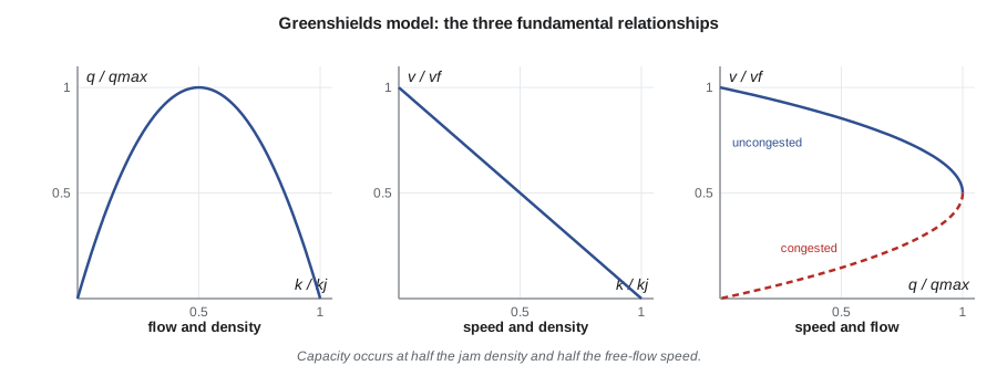
The flow-density curve divides traffic into two regimes. On the left branch, density is below the critical density and traffic is uncongested: adding vehicles increases flow. On the right branch, density is above critical and traffic is congested: adding vehicles reduces flow, because the speed drop outweighs the extra vehicles. Every flow below capacity can occur in two states, one fast and sparse, one slow and dense. This explains why a freeway can carry the same volume at 100 km/h (60 mph) at 6 a.m. and at 30 km/h (20 mph) in a stop-and-go jam at 8 a.m.

Greenshields's linear model is the simplest of many. Real data show that speed stays near the free-flow value over a wide range of low densities, then falls more sharply near capacity; the Highway Capacity Manual's speed-flow curves, used in lesson 5, reflect that shape. Other models include the Greenberg logarithmic model, the Underwood exponential model and the triangular flow-density diagram used in many simulation models. The simple model is still valuable for intuition and for hand calculations like those below.

Shockwaves

When traffic changes from one state to another, for example from fast and sparse to slow and dense, the boundary between the two states moves along the road. This moving boundary is a shockwave. Its speed follows from conservation of vehicles: the number of vehicles entering the boundary from one side must equal the number leaving on the other. If the upstream state has flow \(q_1\) and density \(k_1\), and the downstream state has \(q_2\) and \(k_2\), the shockwave speed is

On a flow-density diagram, \(w\) is the slope of the line joining the two states. A positive \(w\) means the boundary moves downstream, in the direction of traffic; a negative \(w\) means it moves upstream, against traffic. A queue at a red signal grows upstream at a backward shockwave speed; when the light turns green, a second backward wave, the start-up wave, travels through the queue as drivers begin to move.

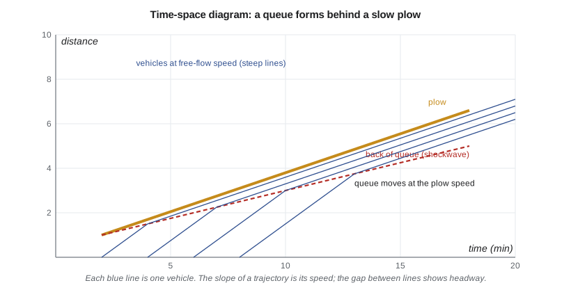
A time-space diagram, which plots vehicle positions against time, is the best way to visualize these waves. Each vehicle's trajectory is a line whose slope is its speed. Where trajectories bend from steep to shallow, vehicles have joined a queue; the line through those bends is the shockwave. Time-space diagrams are also the basic tool for coordinating traffic signals along a corridor, as lesson 6 discusses.

The plow on the northern highway

The highway north of the city is a two-lane road with one lane in each direction, and in snow nobody passes the plow. Upstream of the plow, traffic flows at 900 veh/h. Owen fits the Greenshields model to speed data from the highway's permanent count station, with a free-flow speed of 55 mph and a jam density of 185 veh/mi/ln. The plow travels at 19 mph, and the vehicles behind it are forced into a congested state moving at the plow's speed. The script finds both states and the shockwave between them.

# Greenshields model and a moving bottleneck behind a snowplow
UNITS = "US"
SI = UNITS == "SI"
if SI:
    vf, kj = 88.0, 115.0      # free-flow speed km/h, jam density veh/km/ln
    ul, uk = "km/h", "veh/km/ln"
else:
    vf, kj = 55.0, 185.0      # mph, veh/mi/ln
    ul, uk = "mph", "veh/mi/ln"
qmax = vf * kj / 4
print(f"capacity qmax = {qmax:,.0f} veh/h/ln at k = {kj/2:.0f} {uk}, v = {vf/2:.0f} {ul}")
def k_from_q(q, congested=False):
    # solve q = vf k (1 - k/kj) for k
    disc = max(0.0, 1 - 4 * q / (vf * kj))
    r = disc ** 0.5
    return kj / 2 * (1 + r) if congested else kj / 2 * (1 - r)
# the two-lane highway north of the city: one lane per direction, no passing behind a plow
q1 = 900.0; k1 = k_from_q(q1); v1 = q1 / k1
vp = 30.0 if SI else 19.0               # plow speed
k2 = kj * (1 - vp / vf); q2 = vp * k2   # queue behind the plow: congested branch at the plow speed
w = (q2 - q1) / (k2 - k1)               # shockwave at the back of the queue
print(f"upstream:    q = {q1:,.0f} veh/h, k = {k1:.1f} {uk}, v = {v1:.1f} {ul}")
print(f"behind plow: q = {q2:,.0f} veh/h, k = {k2:.1f} {uk}, v = {vp:.0f} {ul}")
print(f"shockwave speed = {w:.1f} {ul} ({'backward' if w < 0 else 'forward'} relative to the road)")
grow = vp - w
print(f"queue grows at {grow:.1f} {ul}; after 15 min it is {grow/4:.2f} {'km' if SI else 'mi'} long")
print(f"vehicles in the queue after 15 min = {grow/4*k2:.0f}")
# when the plow turns off, the queue discharges at capacity; recovery wave
k3 = kj / 2; q3 = qmax
w3 = (q3 - q2) / (k3 - k2)
print(f"recovery wave after the plow leaves = {w3:.1f} {ul}")

capacity qmax = 2,544 veh/h/ln at k = 92 veh/mi/ln, v = 28 mph
upstream:    q = 900 veh/h, k = 18.1 veh/mi/ln, v = 49.6 mph
behind plow: q = 2,301 veh/h, k = 121.1 veh/mi/ln, v = 19 mph
shockwave speed = 13.6 mph (forward relative to the road)
queue grows at 5.4 mph; after 15 min it is 1.35 mi long
vehicles in the queue after 15 min = 163
recovery wave after the plow leaves = -8.5 mph

Upstream, the 900 veh/h travel at about 50 mph at a density of 18 veh/mi. Behind the plow, the congested state at 19 mph has a density of about 121 veh/mi and a flow of about 2,300 veh/h on the Greenshields curve. The back of the queue moves forward at about 13.6 mph, slower than the plow's 19 mph, so the queue lengthens by about 5.4 mi every hour, reaching 1.35 mi and about 165 vehicles after 15 minutes. When the plow turns off, the queue discharges at capacity and a recovery wave travels backward through it at about 8.5 mph. These numbers explain the city's rule that plows on the two-lane highway pull over at the designated turnouts every 10 minutes or so when traffic builds up behind them.

The same reasoning applies to a lane closure in a work zone, a crash that blocks a lane, a slow truck on a grade, or a signal that turns red. In each case, the engineer identifies the upstream and downstream states, computes the shockwave speeds, and finds how long and how far the queue will extend. That tells the work zone designer where to place the first warning sign, and tells the signal designer whether a queue will spill back through an upstream intersection.

Queueing at a bottleneck

A simpler model is often enough for bottlenecks: the input-output or queueing diagram. If demand \(\lambda\) exceeds the capacity \(\mu\) of a bottleneck for a period \(T\), a queue grows at a rate \(\lambda - \mu\), reaching \((\lambda - \mu)T\) vehicles. After demand falls below capacity, the queue dissipates at \(\mu - \lambda\). The total delay is the area between the cumulative arrival and departure curves. This deterministic model ignores the randomness of arrivals, which lesson 6 adds for signals, but it gives quick answers.