
CIV-390 · Lesson 11 of 12 · 19 min
Road safety analysis
Thirty-one crashes in five years were reported at Ridgeway Road and Carrick Street, more than at any other intersection on the corridor, and residents want to know why the city has not acted. But a count of crashes alone does not say whether an intersection is unusually dangerous: busy intersections have more crashes simply because more vehicles pass through them, and any site's count bounces up and down from year to year by chance. This lesson introduces the modern, statistical approach to road safety analysis: the Safe System philosophy, crash rates, safety performance functions, the Empirical Bayes method, crash modification factors and the economic evaluation of countermeasures.
The Safe System approach
Traditional road safety focused on preventing crashes by changing driver behavior, with education and enforcement. The Safe System approach, which originated in Sweden's Vision Zero and the Netherlands' Sustainable Safety programs in the 1990s, starts from different premises: people will make mistakes, the human body has a limited tolerance to crash forces, and the system should be designed so that mistakes do not lead to death or serious injury. Responsibility is shared among system designers, operators, vehicle makers and users. The US Department of Transportation's National Roadway Safety Strategy, released in 2022, adopts the Safe System approach, and many US cities have adopted Vision Zero plans.
In practice, the Safe System approach emphasizes managing kinetic energy. The risk of death for a pedestrian struck by a car rises steeply with impact speed, from low at 30 km/h (20 mph) to high at 60 km/h (35 to 40 mph) and above. Side impacts at intersections become far more severe above about 50 km/h (30 mph). Hence the Safe System toolbox: lower speeds where people walk, roundabouts instead of high-speed right-angle conflicts, separation of opposing traffic, forgiving roadsides, protected bike lanes and safe crossings. The roundabout in lesson 7 and the road diet in lesson 10 are Safe System measures.
Crash data and crash rates
Crashes are rare, random events, and their analysis must respect that. A crash rate normalizes the count by exposure. For a road segment, the rate is crashes per million vehicle-kilometers (or vehicle-miles) of travel; for an intersection, crashes per million entering vehicles (MEV):
where \(N\) is the number of crashes in \(n\) years. Crash rates allow comparisons between sites of different volumes, but they assume that crashes rise in proportion to traffic, which is generally not true: the relationship is usually non-linear. A rate can make a low-volume site look dangerous on the strength of one or two crashes. These problems led to the methods of the Highway Safety Manual (HSM), first published by AASHTO in 2010, which Canadian and US agencies now use widely.
Severity matters as much as frequency. A site with many minor rear-end crashes is a different problem from one with a few serious pedestrian injuries. Safety programs increasingly focus on fatal and serious injury (FSI) crashes, and use crash cost weighting or separate analyzes for severe crashes, so that a countermeasure that prevents one serious injury is not outranked by one that prevents several fender-benders.
Regression to the mean
Imagine a city selects for treatment the ten intersections with the most crashes last year, installs a countermeasure, and finds that crashes fell by 30 % the following year. Some or all of that fall would have happened anyway: sites are selected because they had an unusually high count, and a high count is partly bad luck that will not repeat. This statistical effect, regression to the mean, has made many ineffective treatments look successful and has wasted money on sites that were not truly dangerous. Any credible safety analysis must account for it.
Safety performance functions
A safety performance function (SPF) is a statistical model that predicts the average number of crashes per year at sites with given characteristics, usually as a function of traffic volume. SPFs are estimated from data on many similar sites, using negative binomial regression because crash counts are more variable than a Poisson model allows. A typical SPF for an intersection has the form
The HSM provides SPFs for rural two-lane roads, rural multilane highways, urban and suburban arterials, freeways and interchange ramps, each for base conditions, with crash modification factors to adjust for features such as lane width, lighting or left-turn phasing, and a calibration factor to match local crash experience. The negative binomial model also gives an overdispersion parameter \(k\), which measures how much real counts scatter around the SPF prediction.
The Empirical Bayes method
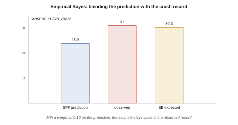
The Empirical Bayes (EB) method combines the SPF prediction with the site's own crash history to estimate the expected number of crashes, correcting for regression to the mean. The expected crashes are a weighted average of the predicted and observed counts:
When the prediction is reliable (small overdispersion) or the site has few predicted crashes, the weight leans toward the prediction; when many crashes are predicted over a long period, the site's own record carries more information and the weight shifts toward it. The difference between the expected and predicted crashes, the excess expected crashes, is the best measure of how much a site could improve, and is used to rank sites in network screening.
Crash modification factors
A crash modification factor (CMF) is the ratio of the expected crashes with a treatment to the expected crashes without it. A CMF of 0.80 means the treatment is expected to reduce crashes by 20 %; a CMF above 1.0 means it increases them. CMFs come from before-after studies (ideally using EB or comparison groups to control for regression to the mean) and cross-sectional studies. They apply to specific crash types and severities, and they carry uncertainty, reported as a standard error. FHWA's CMF Clearinghouse collects published CMFs and rates their quality, and the HSM includes many. When several independent treatments are applied, their CMFs are usually multiplied, though this may overstate the combined effect if the treatments act on the same crashes.
| Treatment | Typical CMF range (total or target crashes) | Notes |
|---|---|---|
| Conversion of a stop-controlled intersection to a roundabout | about 0.2 to 0.6 for injury crashes | Largest benefits for severe crashes |
| Road diet (4 to 3 lanes) | about 0.5 to 0.8 | Depends on volumes and setting |
| Protected or protected-permitted left-turn phasing | about 0.7 to 0.9 | Mainly left-turn crashes |
| Retroreflective signal backplates | about 0.85 | Total crashes at signals |
| Leading pedestrian interval | about 0.85 to 0.9 | Pedestrian-vehicle crashes |
| Median refuge island at an uncontrolled crossing | about 0.5 to 0.7 | Pedestrian crashes |
Analyzing Ridgeway Road and Carrick Street
The intersection had 31 reported crashes in five years. Owen uses an illustrative SPF for urban four-leg signalized intersections with \(a\) = −10.99, \(b\) = 1.07, \(c\) = 0.23 and an overdispersion of 0.39, with AADTs of 18,500 on Ridgeway and 7,200 on Carrick. The crash pattern shows a cluster of left-turn crashes between eastbound left turners and westbound through vehicles, the classic signature of permitted left turns across two opposing lanes. The proposed treatment is protected-permitted left-turn phasing, with an illustrative CMF of 0.84 for total crashes. The script estimates the expected crashes, the crash rate and the benefit-cost ratio of the treatment.
# Network screening and an Empirical Bayes estimate for Ridgeway and Carrick
import math
UNITS = "US"
SI = UNITS == "SI"
years = 5
obs = 31                                 # reported crashes at the intersection in five years
AADT_major, AADT_minor = 18500, 7200
# an illustrative safety performance function for urban four-leg signals (form used in the HSM)
a, b, c = -10.99, 1.07, 0.23
Npred = math.exp(a + b * math.log(AADT_major) + c * math.log(AADT_minor)) * years
k = 0.39                                 # overdispersion parameter of the SPF
w = 1 / (1 + k * Npred)
Nexp = w * Npred + (1 - w) * obs
print(f"predicted (SPF) = {Npred:.1f}, observed = {obs}, weight w = {w:.2f}")
print(f"expected crashes = {Nexp:.1f} in {years} years ({Nexp/years:.1f} per year)")
print(f"excess expected crashes = {Nexp - Npred:.1f}")
mev = (AADT_major + AADT_minor) * 365 * years / 1e6
print(f"crash rate = {obs/mev:.2f} per million entering vehicles")
# treatment: protected left-turn phasing on Ridgeway (illustrative CMF 0.84 for total crashes)
cmf = 0.84
saved = Nexp / years * (1 - cmf)
cost_per_crash = 230000 if SI else 180000      # illustrative average societal cost per crash, local currency
life, i = 15, 0.04
pwf = (1 - (1 + i) ** -life) / i
benefit = saved * cost_per_crash * pwf
cost = 95000 if SI else 75000                  # signal heads, detection, retiming
print(f"crashes reduced = {saved:.2f} per year; present value of benefits = {benefit:,.0f}")
print(f"cost = {cost:,.0f}; benefit-cost ratio = {benefit/cost:.1f}")
# combining two treatments multiplies CMFs (if they act independently)
print(f"with retroreflective backplates too (CMF 0.85): combined CMF = {cmf*0.85:.2f}")predicted (SPF) = 23.9, observed = 31, weight w = 0.10 expected crashes = 30.3 in 5 years (6.1 per year) excess expected crashes = 6.4 crash rate = 0.66 per million entering vehicles crashes reduced = 0.97 per year; present value of benefits = 1,941,562 cost = 75,000; benefit-cost ratio = 25.9 with retroreflective backplates too (CMF 0.85): combined CMF = 0.71
The SPF predicts about 24 crashes in five years for a typical site with these volumes; with 31 observed and a weight of 0.10, the EB estimate is about 30 crashes, or 6.1 a year, about 6 more than a typical site. Because the weight on the prediction is small, the long and fairly large record dominates, and the site really does appear to perform worse than its peers; the excess is concentrated in left-turn crashes. The protected-permitted phasing is expected to prevent about one crash a year. Using an illustrative average comprehensive cost of $180,000 per crash, a 15-year life and a 4 % discount rate, the benefits have a present value of about $1.9 million against a cost of about $75,000, a benefit-cost ratio of about 26. Adding retroreflective backplates to the signal heads would bring the combined CMF to about 0.71. These low-cost signal improvements are clearly worthwhile.
The crash cost is the most uncertain input. Agencies publish their own values, often by severity, and the average cost per crash depends on the mix of severities at the site; a site with a history of serious injuries has a much higher average. Because the benefit-cost ratio here is so high, the conclusion does not depend on the exact value, which is a useful kind of robustness to report.
Worked problem
Crash rate of a segment
The 0.75 mi section of Ridgeway between Carrick Street and the school had 14 crashes in 5 years with an AADT of 18,500. Find the rate per million vehicle-miles.
Show solution
- \[\text{exposure} = 18\,500 \times 365 \times 5 \times 0.75 / 10^6 = 25.3\ \text{million veh-mi}\]
- \[R = 14/25.3 = 0.55\ \text{per million veh-mi}\]
Answer: The rate is useful for comparison with similar segments, but by itself it says nothing about regression to the mean or the non-linear effect of volume; the EB method is the better basis for ranking.
Systemic safety and road safety audits
Not all safety work responds to crash history. Many severe crashes, especially on rural roads and involving pedestrians, are spread thinly over a network, so no single site stands out. The systemic approach identifies risk factors associated with severe crashes, such as horizontal curves without shoulders, unlit crossings on multilane roads, or high-speed left turns, and treats all sites with those features, before crashes occur. The horizontal curve on the old Ridgeway extension, with its winter run-off-road history and sharp radius, fits a systemic risk profile even though its crash count is modest.
A road safety audit is a formal, independent review of a project's safety by a team not involved in its design, at stages from planning to opening. FHWA promotes road safety audits as a proven safety countermeasure, and many states require them for major projects. The team arranges an audit of the Ridgeway designs at the preliminary design stage, so that issues can be fixed cheaply on paper.
Common mistakes
MistakeRanking sites by crash count alone.
InsteadUse the EB expected crashes or excess expected crashes to account for volume and regression to the mean.
MistakeCrediting a treatment with the whole drop in crashes after selecting a high-crash site.
InsteadPart of the drop is regression to the mean; use EB before-after methods.
MistakeApplying a CMF to crash types it does not affect.
InsteadMatch the CMF to the target crash type and severity, and note its standard error.
MistakeMultiplying CMFs for treatments that act on the same crashes.
InsteadCombined effects may be smaller than the product; use judgment or studies of the combination.
Summary and key terms
- The Safe System approach designs for human error and limits crash energy to survivable levels.
- Crash rates normalize by exposure but assume a linear relationship and are distorted by randomness.
- Safety performance functions predict average crashes for similar sites; EB blends prediction and history with \(w = 1/(1 + kN_{pred})\).
- Crash modification factors quantify treatment effects; benefit-cost analysis compares crash savings with costs.
- Systemic safety and road safety audits address risk before crashes occur.
- Safe System approach
- A philosophy that designs roads so that human errors do not cause death or serious injury.
- Regression to the mean
- The tendency of an unusually high count to be followed by a lower one by chance.
- Safety performance function
- A model predicting average crash frequency from traffic volume and site features.
- Empirical Bayes method
- A method that combines an SPF prediction with observed crashes to estimate expected crashes.
- Crash modification factor
- The ratio of expected crashes with a treatment to those without it.
- Network screening
- The process of ranking sites in a network by their potential for safety improvement.
- Road safety audit
- An independent formal review of a road project's safety.
Practice problems
Work each problem on paper first, then reveal the answer to check.
An intersection has AADTs of 12,000 and 4,000 and 18 crashes in 3 years. Find the rate per MEV.
Show answer
\(18 \times 10^6/(365 \times 3 \times 16\,000) = 1.03\) per MEV.
An SPF predicts 10 crashes over five years with k = 0.5, and 16 were observed. Find the EB estimate.
Show answer
\(w = 1/(1 + 5) = 0.167\); \(N_{exp} = 0.167(10) + 0.833(16) = 15.0\).
Two independent treatments have CMFs of 0.80 and 0.90. Estimate the combined reduction.
Show answer
\(0.80 \times 0.90 = 0.72\): about 28 %.
Why does a long crash record shift the EB weight toward the observed count?
Show answer
Over more years the predicted count grows, so \(w = 1/(1 + kN_{pred})\) falls and the site's own record carries more weight.
Lesson quiz · 5 questions
Score 60% or more to complete this lesson.
Create a free account to save your progress, take quizzes and earn a certificate.