
CIV-390 · Lesson 12 of 12 · 20 min
Travel demand forecasting and the corridor capstone
Every recommendation in the Ridgeway Road study rests on a forecast: how many vehicles will use the corridor in 20 years, where they will come from, and how they will respond if the road changes. Lesson 1 used a simple growth factor. Planners use travel demand models that represent why people travel, where they go, how they get there and which routes they choose. This final lesson introduces the four-step model, applies its main components to a simplified three-zone version of the city, and then brings together the analyzes of the whole course into the corridor recommendations that Kestrel Bay presents to the city.
Why model travel demand?
Travel is a derived demand: people travel to reach activities such as work, school and shopping, not for its own sake. Changes to the transportation system, such as a new road, better transit or a road diet, change the time and cost of reaching those activities, and people respond by changing route, mode, time of travel, destination or even whether they make the trip. Growth factor forecasts cannot capture these responses. A travel demand model represents the region as zones, the network of roads and transit links between them, and a set of behavioral relationships, and predicts the flows on each link for a future year and set of policies.
In the United States, every urbanized area with more than 50,000 people has a metropolitan planning organization (MPO) responsible for a long-range transportation plan, and most MPOs maintain a regional travel demand model. The Duluth-Superior Metropolitan Interstate Council is the MPO for the Duluth area. The models are calibrated to household travel surveys and counts, and their forecasts are only as good as the land-use projections that feed them.
The four-step model
The classic urban travel demand model has four sequential steps. Trip generation estimates the number of trips produced by and attracted to each zone, from land use and household characteristics. Trip distribution links productions and attractions into a table of trips between zone pairs. Mode choice splits each zone-pair flow among modes such as car, transit, walking and cycling. Traffic assignment loads the trips onto the network, finding the routes and link volumes. Because congestion affects travel times, which in turn affect distribution and mode choice, practical models feed the assigned travel times back to the earlier steps and iterate until they are consistent.
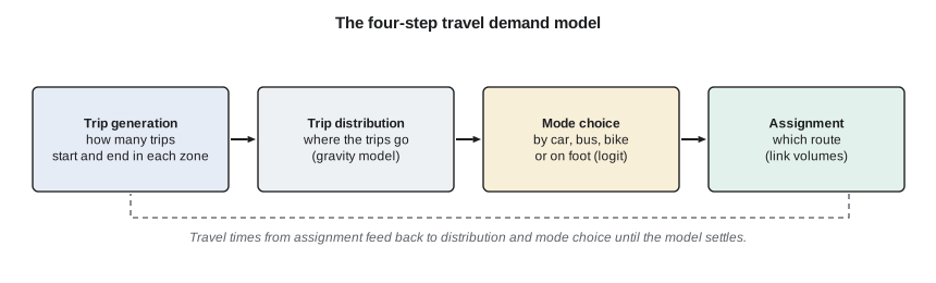
Many large regions have moved to activity-based models, which simulate the daily activity schedules of synthetic individuals and households, and to dynamic traffic assignment, which represents queues over time. The four-step framework remains the foundation for understanding them and is still used in many mid-sized cities.
Trip generation
Trip generation models relate trips to their causes. Productions, usually the home end of trips, are estimated from household size, income, vehicle ownership and other characteristics, often by cross-classification: trip rates per household are tabulated by household type and multiplied by the number of households of each type. Attractions, the non-home end, are estimated from employment and floor area by sector. Because every trip has two ends, the total attractions are scaled to match the total productions for each trip purpose. For individual developments, engineers use trip rates from the Institute of Transportation Engineers' Trip Generation Manual, now in its eleventh edition, which tabulates rates per unit of floor area, dwelling or employee for many land uses, with local adjustments for transit, walking and mixed use.
Trip distribution: the gravity model
The gravity model, by analogy with Newton's law, states that the number of trips between zones is proportional to the productions of the origin and the attractions of the destination, and decreases with the travel time or cost between them:
where \(F_{ij}\) is a friction factor that declines with travel time, often a power function \(t_{ij}^{-b}\) or an exponential \(e^{-\beta t_{ij}}\), and the denominator ensures that all trips produced in zone \(i\) are distributed. The friction factors are calibrated so that the model reproduces the observed distribution of trip lengths. A doubly constrained version also balances the attractions at each destination by iteration.
Mode choice: the logit model
Mode choice is modeled with discrete choice theory. Each mode \(m\) has a utility \(U_m\), a linear function of its travel time, waiting time, cost and other attributes, plus a mode-specific constant capturing unmeasured preferences such as comfort or reliability. If the unobserved parts of utility follow a particular extreme-value distribution, the probability of choosing mode \(m\) is given by the multinomial logit model:
The coefficients are estimated from survey data on actual choices. The ratio of the time and cost coefficients gives the value of travel time implied by the model. Logit models predict how mode shares change when service changes: for example, how much transit ridership rises if waiting time falls because buses run more often. Waiting time is usually weighted more heavily than in-vehicle time, because people dislike waiting.
Traffic assignment
Assignment loads the trip table onto the network. The simplest method, all-or-nothing assignment, puts every trip on the shortest path; it ignores congestion. Equilibrium assignment follows Wardrop's first principle: at equilibrium, no traveler can reduce their travel time by switching routes, so all used routes between an origin and destination have equal travel time. Congestion is represented by link performance functions, the most common being the Bureau of Public Roads (BPR) function:
where \(t_0\) is the free-flow travel time and \(v/c\) the volume-to-capacity ratio. The fourth power means travel time rises slowly at first and sharply as volume approaches and exceeds capacity. The function is a planning approximation; operational detail at intersections comes from the methods of lessons 6 and 7.
A three-zone model of the corridor
Sofia builds a teaching model with three zones: the North end, mostly housing; Downtown, with most jobs; and the Ridgeway area, with the operations site and the retail plaza. Productions for home-based work trips in the PM peak period come from households, attractions from jobs, and the friction factor is \(t^{-1.8}\). For mode choice between the North end and Ridgeway, the car takes 15 minutes and costs $4.50 for fuel and parking; the bus takes 26 minutes in the vehicle, costs $3.00 and has an average wait of half the headway. The script also applies the BPR function to the corridor's two sections under the recommended cross-sections.
# Four-step model for three zones and a BPR check on Ridgeway Road
import math
UNITS = "US"
SI = UNITS == "SI"
zones = ["North (homes)", "Downtown", "Ridgeway (operations, retail)"]
households = [5200, 2100, 900]
jobs = [600, 7400, 2300]
P = [h * 1.6 for h in households]        # PM-peak home-based work productions (trip rate 1.6 per household per day scaled to peak)
A = [j * 1.0 for j in jobs]
A = [a * sum(P) / sum(A) for a in A]     # balance attractions to productions
t = [ [4, 12, 15], [12, 3, 9], [15, 9, 4] ]  # zone-to-zone travel time, min
F = lambda m: m ** -1.8                  # friction factor
T = [ [P[i] * A[j] * F(t[i][j]) / sum(A[k] * F(t[i][k]) for k in range(3)) for j in range(3)] for i in range(3) ]
print("trip table (home-based work, PM peak period):")
for i in range(3):
    print(f"  {zones[i]:30s} " + "  ".join(f"{x:7.0f}" for x in T[i]))
# binary logit mode choice for the North -> Ridgeway pair
def Ucar(time, cost): return -0.025 * time - 0.30 * cost
def Ubus(time, cost, wait): return -1.20 - 0.025 * time - 0.30 * cost - 0.05 * wait
uc = Ucar(15, 4.50); ub = Ubus(26, 3.00, 10)
pb = math.exp(ub) / (math.exp(uc) + math.exp(ub))
print(f"bus share North -> Ridgeway = {pb*100:.1f} %; with 15-min service instead of 30-min: ", end="")
ub2 = Ubus(26, 3.00, 7.5); pb2 = math.exp(ub2) / (math.exp(uc) + math.exp(ub2))
print(f"{pb2*100:.1f} %")
# BPR link performance on the Ridgeway corridor (peak direction)
L = 2.8 if SI else 1.75
v0 = 50.0 if SI else 31.0                # free-flow travel speed on the corridor
t0 = L / v0 * 60
for name, vol, cap in (("west, four lanes today", 1200, 1950), ("west, four lanes design", 1447, 1950), ("east, three lanes design", 865, 990), ("east, three lanes, +20 %", 1040, 990)):
    tt = t0 * (1 + 0.15 * (vol / cap) ** 4)
print(f"{name:26s} v/c {vol/cap:.2f} travel time {tt:.1f} min (free flow {t0:.1f})")trip table (home-based work, PM peak period): North (homes) 2717 4638 965 Downtown 21 3201 138 Ridgeway (operations, retail) 20 608 813 bus share North -> Ridgeway = 17.9 %; with 15-min service instead of 30-min: 19.8 % west, four lanes today v/c 0.62 travel time 3.5 min (free flow 3.4) west, four lanes design v/c 0.74 travel time 3.5 min (free flow 3.4) east, three lanes design v/c 0.87 travel time 3.7 min (free flow 3.4) east, three lanes, +20 % v/c 1.05 travel time 4.0 min (free flow 3.4)
The gravity model sends most North-end trips Downtown, as expected, and about 965 to the Ridgeway zone. The logit model gives the bus about an 18 % share between the North end and Ridgeway with 30-minute service, rising to about 20 % if the bus ran every 15 minutes. The share rises only modestly because in-vehicle time and the bus constant also matter; frequency alone will not empty the road, but it helps, especially for students and shift workers at the operations site who do not drive. The BPR check shows that the west section with four lanes stays close to free-flow travel time in the design year, and the east section with three lanes adds about 20 seconds at a v/c of 0.87. If traffic grew 20 % faster than forecast, the east section would reach a v/c of about 1.05, and travel time across it would rise to about 4.0 minutes. That is the main risk of the road diet, and it is modest.
Worked problem
Logit mode share
Car utility is −1.2 and bus utility is −2.4 for a trip. Find the bus share. If a new express route raises the bus utility by 0.5, what is the new share?
Show solution
- \[P_{bus} = \frac{e^{-2.4}}{e^{-1.2} + e^{-2.4}} = \frac{0.0907}{0.3012 + 0.0907} = 0.231\]
- \[P'_{bus} = \frac{e^{-1.9}}{e^{-1.2} + e^{-1.9}} = \frac{0.1496}{0.3012 + 0.1496} = 0.332\]
Answer: The bus share rises from 23 % to 33 %. The same utility change has its largest effect when shares are near 50 %, and little effect on a mode with a very small or very large share.
Induced and diverted demand
Models and experience agree that changes in road capacity change demand. Adding lanes to a congested road lowers travel time at first, which attracts trips from other routes, other times and other modes, and over years encourages more and longer trips and more dispersed development: induced demand. Removing capacity has the reverse effect. Some traffic diverts, some shifts in time or mode, and some trips are not made, so traffic 'evaporation' is often larger than simple diversion models predict. For the Ridgeway road diet, the team assumes 10 % diversion on the east section, a cautious value, and checks in lesson 5 that the bypass could absorb it.
The corridor recommendations
Priya's team now assembles the evidence from the whole course into a set of recommendations for the city. Each element answers a problem identified earlier, and each is supported by a calculation and a statement of its assumptions and risks.
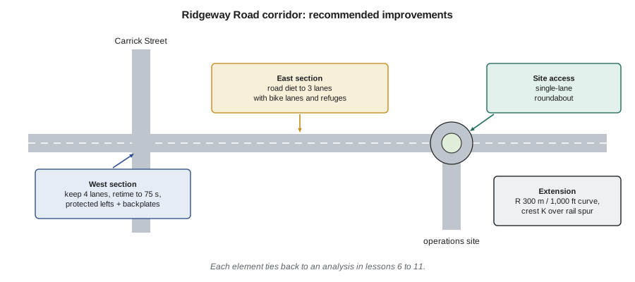
| Element | Recommendation | Basis | Main risk or follow-up |
|---|---|---|---|
| Carrick Street signal | 75 s cycle, protected-permitted lefts, leading pedestrian interval, backplates | Lessons 6 and 11: LOS B and C; B/C about 26 | Monitor queues after opening |
| West section | Keep four lanes; coordinate signals at the posted speed | Lesson 10: one lane would fail (v/c 1.16) | Revisit if demand falls |
| East section | Road diet to three lanes with bike lanes and refuge islands | Lessons 10 and 12: v/c 0.77 to 0.87 | Higher growth could reach v/c 1.05 |
| Operations site access | Single-lane roundabout with truck apron and raised crossings | Lesson 7: LOS B on all entries; stop control fails | Snow storage, accessible crossings |
| Rural extension | Realign to a 1,000 ft curve and a 500 ft crest over the rail spur | Lessons 8 and 9: SSD and sight offset met | Rock cut and rail approvals |
| Bypass freeway | No change now; plan for a third lane or demand management | Lesson 5: LOS E in design year | Diverted traffic adds pressure |
The recommendations are deliberately mixed. They keep capacity where the analysis shows it is needed, reallocate space where it is not, and use the safest intersection form where a new access is built. They also reflect the public's concerns: the left turn out of the plaza is addressed by the protected-permitted phasing and the roundabout at the east end gives drivers a safe place to turn around; the students' crossing gets a refuge island and a leading pedestrian interval. Costs and phasing are set out in the report, with the low-cost signal changes first.
Finally, the report is honest about uncertainty. It states the growth assumptions, shows the sensitivity of the key decision (the road diet) to faster growth, identifies the inputs from guides and research that are approximate (such as the CMFs and crash costs) and recommends monitoring: counts, travel times, speeds and crashes before and after each change, analyzed with the methods of lessons 4 and 11. A transportation engineer's job does not end with construction; it continues as the road is used, measured and adjusted.
Common mistakes
MistakeRunning the four steps once without feedback.
InsteadFeed congested travel times back to distribution and mode choice and iterate to consistency.
MistakeTreating model output as precise.
InsteadReport the assumptions, test sensitivity and present ranges for key decisions.
MistakeIgnoring induced and diverted demand.
InsteadCapacity changes alter route, time, mode and trip making; account for these responses.
MistakeRecommending without monitoring.
InsteadMeasure before and after each change and adjust the design if outcomes differ from forecasts.
Summary and key terms
- Travel is a derived demand; models represent zones, networks and behavioral responses.
- The four-step model: trip generation, distribution, mode choice and assignment, with feedback.
- The gravity model distributes trips by attraction and travel time; the logit model splits trips among modes by utility.
- Equilibrium assignment with BPR link functions loads trips onto routes; capacity changes induce or reduce demand.
- Good recommendations tie each element to analysis, state assumptions and risks, and include monitoring.
- Derived demand
- Demand for travel that arises from the need to reach activities.
- Trip generation
- The step that estimates trips produced by and attracted to each zone.
- Gravity model
- A distribution model in which trips rise with attractions and fall with travel time.
- Logit model
- A discrete choice model giving each mode's share from its utility.
- User equilibrium
- The state in which no traveler can reduce travel time by changing route.
- BPR function
- A link performance function relating travel time to the volume-to-capacity ratio.
- Induced demand
- Additional travel generated by an increase in road capacity.
Practice problems
Work each problem on paper first, then reveal the answer to check.
Zone 1 produces 1,000 trips. Zones A and B attract 600 and 400 trips, with friction factors 0.5 and 1.0. Distribute the trips.
Show answer
\(A F\): 300 and 400; total 700. \(T_{1A} = 1000 \times 300/700 = 429\); \(T_{1B} = 571\).
Car utility is −0.8, bus −1.6 and walk −2.5. Find the three shares.
Show answer
\(e^{U}\): 0.449, 0.202, 0.082; total 0.733. Shares: car 61 %, bus 28 %, walk 11 %.
A link has a free-flow time of 6 min. Find the BPR time at v/c = 0.8 and 1.2.
Show answer
\(6(1 + 0.15 \times 0.41) = 6.4\) min; \(6(1 + 0.15 \times 2.07) = 7.9\) min.
Why might a road diet reduce total traffic rather than only divert it?
Show answer
Some trips change time, mode or destination, or are combined or not made, when the corridor becomes slower for driving.
Lesson quiz · 5 questions
Score 60% or more to complete this lesson.
Create a free account to save your progress, take quizzes and earn a certificate.