
CIV-370 · Lesson 8 of 12 · 19 min
Abstractions, infiltration and the curve number method
Not all the rain that falls on a watershed reaches the creek during a storm. Some is caught by leaves and evaporates, some fills puddles and depressions, and much of it soaks into the soil. These losses are called abstractions, and what remains, the rainfall excess or effective rainfall, becomes direct runoff. Estimating the abstractions is the step that most affects a flood estimate, and it is also the step that development changes most dramatically: a roof or a parking lot abstracts almost nothing. This lesson examines the physics of infiltration and the curve number method, the empirical tool that most North American practice uses to estimate runoff volume.
Interception and depression storage
Interception by vegetation typically removes the first one or two millimeters of a storm, more under dense conifers and less on grass, and matters mainly for small storms. Depression storage, the water held in hollows on the ground and puddles on pavement, ranges from about 1 to 2 mm on smooth pavement to 5 mm or more on lawns and forest floors. Both are filled early in a storm and are often lumped with early infiltration as an initial abstraction.
Infiltration
Infiltration is the passage of water through the soil surface. Its rate depends on the soil texture and structure, the vegetation cover, the moisture already in the soil, frost and the intensity of the rain. The infiltration capacity of a soil is the maximum rate at which it can absorb water. At the start of a storm on dry soil, the capacity is high, because strong suction gradients draw water into the dry pores. As the soil wets, the capacity falls toward a steady value close to the saturated hydraulic conductivity. When the rainfall intensity exceeds the infiltration capacity, the surface ponds and the excess runs off. This mechanism, called infiltration-excess or Hortonian overland flow, dominates on paved surfaces, compacted soils and clayey ground. In humid forests with permeable soils, much runoff instead comes from areas near streams that saturate from below, called saturation-excess runoff.
Robert Horton described the decline of infiltration capacity with an exponential equation in the 1930s:
where \(f_0\) is the initial capacity, \(f_c\) the final capacity and \(k\) a decay constant. The Green-Ampt model of 1911 is more physical. It treats the wetting front as a sharp boundary moving down into the soil, with saturated soil above and the initial moisture content below. Its infiltration rate is
where \(K\) is the saturated hydraulic conductivity, \(\psi\) the suction head at the wetting front, \(\Delta\theta\) the moisture deficit and \(F\) the cumulative infiltration. For a constant rain of intensity \(i > K\), ponding begins when the infiltration capacity falls to \(i\), after a cumulative infiltration \(F_p = K\psi\Delta\theta/(i - K)\). Published tables give Green-Ampt parameters by soil texture, from sand, with a conductivity of over 100 mm/h, to clay, with less than 1 mm/h.
Frozen ground deserves a special word in a northern climate. Soil that freezes while wet becomes nearly impermeable, and early spring rain on frozen ground or on snow runs off almost completely. Designers in Canada and the northern United States often check a spring condition with greatly reduced infiltration in addition to the summer storm.
The curve number method
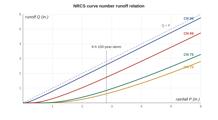
Infiltration models need soil parameters that are rarely measured across a whole watershed. In the 1950s, the US Soil Conservation Service, now the Natural Resources Conservation Service (NRCS), developed a simpler, empirical method from records of rainfall and runoff on small agricultural watersheds. It relates the total runoff depth \(Q\) of a storm to the total rainfall \(P\) through the potential maximum retention \(S\) and an initial abstraction \(I_a\):
The retention is expressed through a dimensionless curve number between about 30 and 100:
A curve number of 100 means no retention, so all rain runs off; lower numbers mean more retention. The method is used across North America and much of the world, and it underlies programs such as HEC-HMS and the NRCS TR-55 and TR-20 procedures. The ratio \(I_a = 0.2S\) has been debated, and analyses of more recent data suggest that a smaller ratio, around 0.05, fits many watersheds better; NRCS documentation discusses the alternative. Designers should use the form their reviewing authority specifies.
Choosing a curve number
The curve number depends on the hydrologic soil group, the land use and cover, the hydrologic condition and the antecedent moisture. NRCS classifies soils into four hydrologic soil groups. Group A soils, such as deep sands, have high infiltration rates; group B soils are moderately fine to moderately coarse; group C soils, such as silty or sandy clay loams and soils with a layer that impedes drainage, have slow infiltration; group D soils, such as clays, soils with a high water table and shallow soils over rock, have very slow infiltration. Soil surveys published by NRCS in the United States, and provincial soil surveys and agricultural databases in Canada, map these groups.
| Cover | A | B | C | D |
|---|---|---|---|---|
| Woods, fair condition | 36 | 60 | 73 | 79 |
| Pasture, good condition | 39 | 61 | 74 | 80 |
| Open space, lawns in good condition | 39 | 61 | 74 | 80 |
| Residential, small lots (about 38 % impervious) | 61 | 75 | 83 | 87 |
| Gravel roads | 76 | 85 | 89 | 91 |
| Impervious: pavement, roofs | 98 | 98 | 98 | 98 |
For a watershed with several land covers, an area-weighted curve number is computed. Strictly, runoff should be computed separately for each cover and the depths weighted, because the relation is nonlinear; averaging curve numbers slightly underestimates runoff from a mix of pavement and lawn. For heavily impervious sites, it is better to treat the directly connected impervious area separately.
The tabulated values apply to average antecedent moisture, called condition II. For dry conditions (I) and wet conditions (III), conversion formulas adjust the curve number; for condition III,
The Kestrel Creek watershed
Owen digitizes the watershed's land cover from air photos and the soils from the NRCS soil survey, which classifies most of the area as a silty glacial lake deposit over till, hydrologic group C. More than half the watershed is mixed forest, about a third is pasture and hay, a tenth is residential lots along the township road and the rest is roads and gravel.
Worked problem
Runoff from the 6-hour, 100-year storm
The area-weighted curve number of the watershed is 75. Find the runoff depth from the 6-hour, 100-year storm of 2.82 in.
Show solution
- Retention and initial abstraction:
- \[S = \frac{1000}{75} - 10 = 3.33\ \text{in.} \qquad I_a = 0.2(3.33) = 0.67\ \text{in.}\]
- Runoff depth:
- \[Q = \frac{(2.82 - 0.67)^2}{2.82 - 0.67 + 3.33} = \frac{4.62}{5.48} = 0.84\ \text{in.}\]
Answer: About 30 % of the storm rainfall becomes direct runoff. The rest is abstracted by interception, depressions and infiltration into the forest and pasture soils.
Sofia's script evaluates the Horton curve and cumulative infiltration for a silt loam, the Green-Ampt ponding time for a steady rain, the area-weighted curve number, the runoff for three storm depths, the site before and after development, and the effect of wet antecedent conditions.
# Abstractions: Horton and Green-Ampt infiltration, and NRCS curve number runoff
from math import exp, log
UNITS = "US"
SI = UNITS == "SI"
f = 1.0 if SI else 1 / 25.4; u = "mm" if SI else "in."; d = 1 if SI else 2
# Horton: f(t) = fc + (f0 - fc) e^(-kt), silt loam (illustrative parameters, mm/h)
f0, fc, kh = 75.0, 10.0, 4.0
print("Horton infiltration capacity (" + ("mm/h" if SI else "in./h") + ")")
for t in (0, 0.25, 0.5, 1, 2, 3):
    print(f"  t = {t:4.2f} h  f = {(fc + (f0 - fc) * exp(-kh * t)) * f:6.{d}f}")
F3 = fc * 3 + (f0 - fc) / kh * (1 - exp(-kh * 3))
print(f"Cumulative infiltration in 3 h: {F3 * f:.{d}f} {u}")
# Green-Ampt ponding time for a constant rain of 30 mm/h on silt loam
K, psi, dth, ir = 6.5, 167.0, 0.30, 30.0       # mm/h, mm suction head, moisture deficit, mm/h
Fp = K * psi * dth / (ir - K); tp = Fp / ir
print(f"Green-Ampt: ponding after Fp = {Fp * f:.{d}f} {u}, at t = {tp * 60:.0f} min")
# NRCS curve number method
def runoff(P, CN):                            # P and result in mm
    S = 25400 / CN - 254; Ia = 0.2 * S
    return 0.0 if P <= Ia else (P - Ia) ** 2 / (P - Ia + S)
shed = [("Mixed forest, fair, soil group C", 0.55, 73), ("Pasture and hay, good, C", 0.30, 74),
        ("Residential, small lots, C", 0.10, 83), ("Roads and gravel, C", 0.05, 89)]
CN = sum(a * c for _, a, c in shed)
print("\nKestrel Creek watershed land cover:")
for name, a, c in shed: print(f"  {name:36s} {a * 100:4.0f} %  CN {c}")
print(f"Area-weighted CN = {CN:.1f} -> use {round(CN)}")
CN = round(CN)
P100 = 71.5                                   # 6-hour 100-year depth from lesson 7, mm
for P in (30.0, 50.0, P100):
    print(f"  P = {P * f:5.{d}f} {u}: S = {(25400 / CN - 254) * f:.{d}f}, Ia = {0.2 * (25400 / CN - 254) * f:.{d}f}, Q = {runoff(P, CN) * f:.{d}f} {u}")
# the site before and after development
pre, post = 70, 89
for lab, c in (("Site before development", pre), ("Site after development", post)):
    q = runoff(P100, c)
    print(f"{lab}: CN {c}, 100-year runoff {q * f:.{d}f} {u} ({q / P100 * 100:.0f} % of rain)")
# antecedent condition: wet (AMC III) curve number
CN3 = 23 * CN / (10 + 0.13 * CN)
print(f"\nWatershed CN {CN} becomes {CN3:.0f} for wet antecedent conditions; Q100 = {runoff(P100, CN3) * f:.{d}f} {u}")Horton infiltration capacity (in./h) t = 0.00 h f = 2.95 t = 0.25 h f = 1.34 t = 0.50 h f = 0.74 t = 1.00 h f = 0.44 t = 2.00 h f = 0.39 t = 3.00 h f = 0.39 Cumulative infiltration in 3 h: 1.82 in. Green-Ampt: ponding after Fp = 0.55 in., at t = 28 min Kestrel Creek watershed land cover: Mixed forest, fair, soil group C 55 % CN 73 Pasture and hay, good, C 30 % CN 74 Residential, small lots, C 10 % CN 83 Roads and gravel, C 5 % CN 89 Area-weighted CN = 75.1 -> use 75 P = 1.18 in.: S = 3.33, Ia = 0.67, Q = 0.07 in. P = 1.97 in.: S = 3.33, Ia = 0.67, Q = 0.37 in. P = 2.81 in.: S = 3.33, Ia = 0.67, Q = 0.84 in. Site before development: CN 70, 100-year runoff 0.61 in. (22 % of rain) Site after development: CN 89, 100-year runoff 1.73 in. (62 % of rain) Watershed CN 75 becomes 87 for wet antecedent conditions; Q100 = 1.60 in.
Reading the results
The Horton curve falls from 2.95 in./h to near its final value of 0.39 in./h within about an hour; the soil absorbs 1.82 in. in the first three hours if water is always available. The Green-Ampt model shows that a steady rain of 1.2 in./h would pond the surface after only 28 minutes, having infiltrated 0.55 in. The curve number results make the nonlinearity plain: a 1.18 in. storm produces less than 0.1 in. of runoff because most of it is absorbed by the initial abstraction of 0.67 in., while the 2.82 in. storm produces 0.84 in.
Development triples the site's runoff. With a curve number of 70 before development, the 100-year storm produces 0.61 in. of runoff, 22 % of the rain. After development, with 60 % of the site under roofs, pavement and gravel, the curve number rises to 89, and the same storm produces 1.73 in., 62 % of the rain. That extra 1.1 in. over 18.5 acres is about 75,000 ft³ of water that must either be stored and released slowly or infiltrated, and it is the reason for the pond. Wet antecedent conditions matter as much as development: the watershed's curve number of 75 becomes 87, almost doubling the runoff to 1.60 in.
Reducing runoff at the source
Low-impact development, also called green infrastructure, aims to keep runoff closer to its natural volume by infiltrating, evaporating or harvesting rain where it falls. Bioretention cells, permeable pavement, green roofs, vegetated swales and rain gardens all reduce the effective curve number of a site. Many jurisdictions now require developments to retain a specified depth of rainfall on site, such as the first 25 mm or 1 in., in addition to controlling peak flows. At Kestrel Bay, the clay at 4 m depth and the high groundwater limit infiltration, but Anika proposes a vegetated swale along the yard edge and directs the roof drainage of the office building to a rain garden, both of which help with water quality as well as volume.
Practical points
- Map soils and land cover carefully; the curve number controls the runoff volume.
- Compute runoff separately for pervious and impervious areas on developed sites.
- State the antecedent condition used, and check a wet or frozen condition where it matters.
- Use the initial abstraction ratio the reviewing authority specifies.
- Remember that the curve number method gives runoff volume, not the timing; lesson 10 adds timing with a unit hydrograph.
Common mistakes
MistakeAveraging curve numbers for a site with large impervious areas.
InsteadCompute pervious and impervious runoff separately, or the volume will be underestimated.
MistakeApplying the curve number equation to rainfall intensities.
InsteadIt relates storm depths, not rates; apply it to cumulative rainfall.
MistakeUsing summer infiltration parameters for a spring storm on frozen ground.
InsteadFrozen ground can be nearly impermeable; check that case.
MistakeForgetting that runoff is zero until the rainfall exceeds the initial abstraction.
InsteadSmall storms may produce no runoff at all from pervious areas.
Summary and key terms
- Abstractions are interception, depression storage and infiltration; the remainder is rainfall excess.
- Horton: \(f = f_c + (f_0 - f_c)e^{-kt}\); Green-Ampt: \(f = K(1 + \psi\Delta\theta/F)\).
- Curve number: \(Q = (P - I_a)^2/(P - I_a + S)\), \(I_a = 0.2S\), \(S = 25{,}400/CN - 254\) mm or \(1000/CN - 10\) in.
- CN depends on soil group, cover, condition and antecedent moisture.
- Watershed CN 75: 0.84 in. of runoff from the 2.82 in. storm; 1.60 in. with wet conditions.
- Site: CN 70 → 89 raises 100-year runoff from 0.61 to 1.73 in.
- Abstraction
- The part of rainfall that does not become direct runoff.
- Infiltration capacity
- The maximum rate at which a soil can absorb water at a given time.
- Rainfall excess
- The part of rainfall that becomes direct runoff.
- Hortonian overland flow
- Runoff produced when rainfall intensity exceeds the infiltration capacity.
- Curve number
- An empirical parameter of the NRCS method that expresses a watershed's runoff potential.
- Hydrologic soil group
- One of four NRCS soil classes, A to D, based on infiltration rate.
- Antecedent moisture condition
- The wetness of a watershed before a storm.
- Low-impact development
- Practices that manage rainfall close to where it falls to reduce runoff.
Practice problems
Work each problem on paper first, then reveal the answer to check.
Find the runoff from 2.0 in. of rain on a parking lot with CN 98.
Show answer
\(S = 0.204\) in., \(I_a = 0.041\) in., \(Q = (1.959)^2/2.163 = 1.77\) in.
What is the smallest storm that produces any runoff from woods on group B soil (CN 60)?
Show answer
\(S = 6.67\) in., \(I_a = 1.33\) in.; storms smaller than 1.33 in. produce no runoff.
A watershed has CN 70 for average conditions. Find the curve number for wet conditions.
Show answer
\(CN_{III} = 23(70)/(10 + 9.1) = 84\).
Why does development increase runoff more for small storms than the ratio of curve numbers suggests?
Show answer
Pervious areas absorb small storms entirely through the initial abstraction, while impervious surfaces run off almost all of it, so the relative increase is largest for small storms.
Lesson quiz · 5 questions
Score 60% or more to complete this lesson.
Create a free account to save your progress, take quizzes and earn a certificate.