The hydrologic cycle, precipitation and IDF curves

The hydraulics lessons used a design flow of 640 cfs for Kestrel Creek without saying where it came from. Hydrology supplies that number. It is the science of how water moves through the hydrologic cycle, and for the engineer its central question is how much water a storm will deliver to a channel, a culvert or a pond, and how often a storm of that size can be expected. This lesson starts at the beginning, with rain: how it is measured, how its extremes are analyzed statistically, and how intensity-duration-frequency curves turn decades of records into design storms.

The hydrologic cycle

Water evaporates from oceans, lakes and land, and transpires from plants. It condenses into clouds, falls as rain or snow, and then follows one of several paths. Some is intercepted by vegetation and evaporates again. Some infiltrates the soil, where it either returns to the atmosphere through plants, percolates down to recharge groundwater, or moves laterally as interflow to streams. The rest runs off over the surface to channels. Groundwater discharges slowly to streams as baseflow, which keeps creeks running between storms. Rivers carry the water back to lakes and oceans, and the cycle continues.

For a watershed, the cycle can be written as a water balance over any period:

where \(P\) is precipitation, \(R\) is surface runoff, \(G\) is net groundwater outflow, \(ET\) is evapotranspiration and \(\Delta S\) is the change in storage in the soil, snowpack, lakes and aquifers. Over a year, storage changes are small and the balance shows how precipitation divides. Around Duluth, annual precipitation is about 30 in., roughly a fifth or more of it falling as snow; most of it returns to the atmosphere by evapotranspiration, and the rest leaves as streamflow and groundwater. Over a single storm, the balance is dominated by rainfall, infiltration and runoff, and that is the scale engineers usually work at.

The watershed, or drainage basin, is the area that drains to a given point on a stream. Its boundary, the drainage divide, follows the ridges between streams and is traced on topographic maps or, today, from digital elevation models produced from lidar. For Kestrel Creek at the access road, the watershed covers 2.5 mi² of mixed forest, pasture and rural lots, a little larger than the area tributary to the creek's mouth reach downstream.

Precipitation

Precipitation forms when moist air rises and cools. The lifting may be convective, as in the summer thunderstorms that produce short, intense bursts of rain over small areas; frontal, as in the long, widespread rains of autumn and spring storms; or orographic, where air is forced over hills. Lake Superior adds its own effects: lake-effect snow in early winter and enhanced convection in summer. For small watersheds and urban drainage, the short, intense convective storms usually govern the design; for large rivers, long frontal storms and snowmelt do.

Rainfall is measured by gauges. Standard gauges are read once a day; recording gauges, now mostly tipping-bucket instruments, record the time of every small increment and so give intensities over short durations, which are what drainage design needs. The National Weather Service and cooperating observers operate the national network, and the records of stations such as Duluth airport underpin the region's design rainfall. Weather radar estimates rainfall over wide areas, and is valuable for studying the spatial pattern of storms, but must be calibrated against gauges.

A gauge measures rain at a point. Over a watershed, the average depth of a storm is less than the point depth at its center, because storms have finite size. Areal reduction factors convert point rainfall to watershed averages; they are close to 1 for watersheds of a few square kilometers, like Kestrel Creek, and fall significantly for watersheds of hundreds of square kilometers. The average over a watershed from several gauges is estimated by the arithmetic mean, Thiessen polygons or isohyets.

Return period and risk

Engineers describe the rarity of a storm or flood by its annual exceedance probability \(p\), the chance that it will be equalled or exceeded in any one year, or by its return period \(T = 1/p\). A 100-year storm has a 1 % chance of occurring in any year. It does not occur once every 100 years like clockwork: it can occur twice in a decade or not at all in two centuries. The probability that it will be exceeded at least once in \(n\) years is

Over the 50-year design life of a building, the chance of experiencing at least one 100-year storm is \(1 - 0.99^{50} = 39\) %. That figure surprises many clients and is worth explaining to them. It is also why critical facilities, such as the emergency access road at Kestrel Bay, are often checked against rarer events or climate-adjusted ones.

Frequency analysis of rainfall

To estimate the depth of a storm with a given return period at a station, hydrologists extract from the record the largest depth in each year for each duration of interest, such as 5, 10, 15 and 30 minutes and 1, 2, 6, 12 and 24 hours. This annual maximum series is then fitted with a probability distribution, and the fitted distribution is used to read depths for the return periods needed. The Gumbel distribution, the type I extreme value distribution, has long been used for rainfall in Canada and elsewhere. Fitted by the method of moments, it gives the depth for return period \(T\) as

where \(\bar{x}\) and \(s\) are the mean and standard deviation of the annual maxima and \(K_T\) is the frequency factor. For \(T = 100\) years, \(K_T = 3.137\). Some agencies use other distributions, such as the generalized extreme value distribution, and other fitting methods, such as L-moments, particularly when combining data from several stations in a regional analysis.

A record of 30 years gives a fair estimate of the 10-year storm but a very uncertain estimate of the 100-year storm, because the fit must be extrapolated well beyond the data. Regional analysis, which pools records from many stations in a climatically similar area, reduces that uncertainty, and is the basis of the most widely used design atlases.

Intensity-duration-frequency curves

The results of frequency analyses for all durations at a station are summarized in an intensity-duration-frequency (IDF) table and curves: for each return period, the average rainfall intensity is plotted against duration. Intensity falls steeply with duration, because the most intense part of a storm lasts only a few minutes. IDF data are commonly fitted with an equation of the form

with \(t\) in minutes and constants \(a\), \(b\) and \(c\) for each return period. Municipal design standards often publish these constants.

In the United States, NOAA Atlas 14 is the standard source of design rainfall; its volume covering the Midwestern states, including Minnesota, was published in 2013 and gives depths for durations from 5 minutes to 60 days and return periods from 1 to 1,000 years, with confidence limits, through the Precipitation Frequency Data Server. Because Atlas 14 assumes a stationary climate, NOAA is developing Atlas 15, a nationwide replacement that will include projections of future change; a pilot for one state was released in 2024, and preliminary nationwide estimates were scheduled for 2026 for review. Until local criteria adopt Atlas 15, designers in Minnesota use Atlas 14 as the reviewers require.

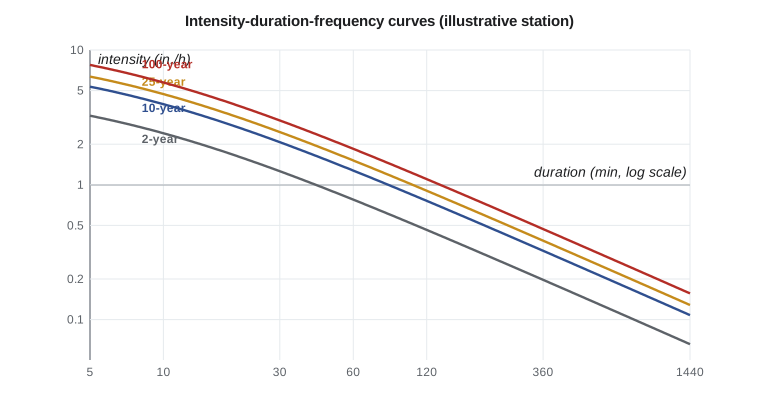
For this course, the team uses an illustrative IDF relation for a station near the site, with \(a = 1340\), \(b = 6\) and \(c = 0.80\) for the 100-year storm in millimeters per hour, converted to inches per hour, and ratios for the other return periods. These values are invented for teaching; an actual design uses the published data.

Design storms

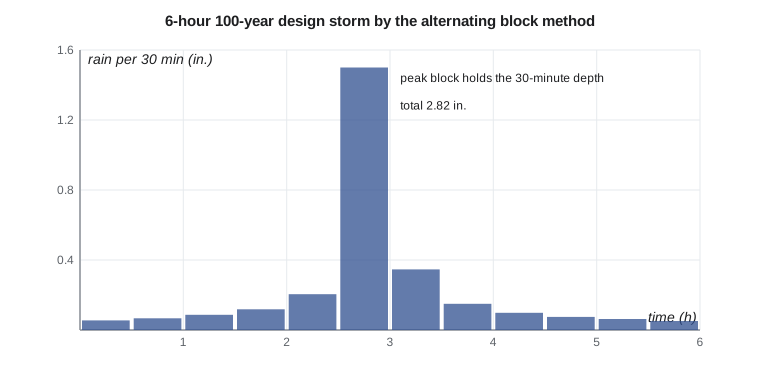
The rational method of lesson 9 needs only an intensity from the IDF curve. Methods that compute a full runoff hydrograph, such as the unit hydrograph of lesson 10, need a design storm: a hyetograph showing how the rain is distributed in time. Several approaches are used. The alternating block method builds a storm directly from the IDF curve: it computes the depth for each duration, takes the increments for successive time blocks, and arranges them with the largest at the center and the others alternating on either side in decreasing order. The resulting storm contains, within it, the IDF depth for every duration. The Chicago storm, developed in the 1950s, gives a smooth equivalent. Standard dimensionless distributions are also used: the NRCS 24-hour distributions in the United States, now often replaced by distributions derived from Atlas 14 data, and in Canada the SCS type II distribution and storm shapes derived from Canadian rainfall records, as municipal standards specify.

Sofia's script fits the Gumbel distribution to the series, tabulates the IDF relation for six return periods and builds a 6-hour, 100-year alternating block storm in 30-minute blocks for use in lessons 8 and 10.

# Rainfall frequency: Gumbel fit to annual maximum 1-hour rainfall, an IDF formula and a design storm
from math import log, sqrt, pi, exp
UNITS = "US"
# Illustrative 30-year series of annual maximum 1-hour rainfall at a station near the site (mm)
amax = [18.2, 24.6, 15.1, 31.8, 20.4, 17.6, 27.3, 22.9, 13.8, 35.4, 19.7, 21.2, 16.4, 29.1, 23.8,
        14.9, 26.0, 19.0, 38.6, 21.7, 17.1, 25.3, 20.8, 30.2, 16.0, 22.4, 18.9, 33.0, 24.1, 19.5]
f = 1.0 if UNITS == "SI" else 1 / 25.4            # mm or inches
u = "mm" if UNITS == "SI" else "in."
x = [v * f for v in amax]
n = len(x); mean = sum(x) / n
sd = sqrt(sum((v - mean) ** 2 for v in x) / (n - 1))
print(f"n = {n}, mean = {mean:.2f} {u}, standard deviation = {sd:.2f} {u}")
def KT(T):                                        # Gumbel frequency factor (method of moments)
    return -sqrt(6) / pi * (0.5772 + log(log(T / (T - 1))))
print("Return period  K_T    1-h depth")
for T in (2, 5, 10, 25, 50, 100):
    print(f"{T:8d}     {KT(T):5.3f}  {mean + KT(T) * sd:7.2f} {u}")
# IDF relation i = a / (t + b)^c for the 100-year storm, t in minutes (fitted to the station's published table)
a, b, c = 1340.0, 6.0, 0.80                       # i in mm/h
scale = {2: 0.42, 5: 0.58, 10: 0.69, 25: 0.82, 50: 0.91, 100: 1.00}
def i(t, T=100): return scale[T] * a / (t + b) ** c * f
ui = "mm/h" if UNITS == "SI" else "in./h"
print(f"\nIntensity ({ui}) by duration and return period")
print("  t(min) " + "".join(f"{T:>8d}" for T in scale))
for t in (5, 10, 15, 30, 60, 120, 360, 720, 1440):
    print(f"{t:8d} " + "".join(f"{i(t, T):8.2f}" for T in scale))
d = 1 if UNITS == "SI" else 2
print(f"100-year depths: 1 h {i(60):.{d}f}, 6 h {i(360) * 6:.{d}f}, 24 h {i(1440) * 24:.{d}f} {u}")
# 6-hour alternating block design storm with 30-minute blocks
dt = 30; N = 12
cum = [i(dt * k) * dt * k / 60 for k in range(1, N + 1)]
inc = [cum[0]] + [cum[k] - cum[k - 1] for k in range(1, N)]
order = sorted(range(N), key=lambda j: -inc[j])
blocks = [0.0] * N; mid = N // 2 - 1
pos = [mid + ((k + 1) // 2) * (1 if k % 2 else -1) for k in range(N)]
for j, p in zip(order, pos): blocks[p] = inc[j]
print(f"\n6-hour 100-year alternating block storm ({u} per 30 min):")
print(" ".join(f"{v:.1f}" if UNITS == "SI" else f"{v:.2f}" for v in blocks))
print(f"total {sum(blocks):.1f} {u}, peak block {max(blocks):.1f} {u}" if UNITS == "SI" else f"total {sum(blocks):.2f} {u}, peak block {max(blocks):.2f} {u}")

n = 30, mean = 0.90 in., standard deviation = 0.25 in.
Return period  K_T    1-h depth
       2     -0.164     0.86 in.
       5     0.719     1.08 in.
      10     1.305     1.22 in.
      25     2.044     1.41 in.
      50     2.592     1.55 in.
     100     3.137     1.68 in.

Intensity (in./h) by duration and return period
  t(min)        2       5      10      25      50     100
       5     3.25    4.49    5.35    6.35    7.05    7.75
      10     2.41    3.33    3.96    4.71    5.22    5.74
      15     1.94    2.68    3.19    3.79    4.20    4.62
      30     1.26    1.74    2.07    2.46    2.73    3.00
      60     0.78    1.07    1.27    1.52    1.68    1.85
     120     0.46    0.64    0.76    0.90    1.00    1.10
     360     0.20    0.27    0.32    0.38    0.43    0.47
     720     0.11    0.16    0.19    0.22    0.25    0.27
    1440     0.07    0.09    0.11    0.13    0.14    0.16
100-year depths: 1 h 1.85, 6 h 2.82, 24 h 3.75 in.

6-hour 100-year alternating block storm (in. per 30 min):
0.06 0.07 0.09 0.12 0.21 1.50 0.35 0.15 0.10 0.07 0.06 0.05
total 2.82 in., peak block 1.50 in.

Reading the results

The IDF table shows the steep fall of intensity with duration: the 100-year intensity is about 7.7 in./h for 5 minutes, 1.85 in./h for an hour and only 0.16 in./h averaged over 24 hours, although the 24-hour depth, 3.75 in., is twice the 1-hour depth. The 6-hour storm totals 2.82 in., and its peak 30-minute block holds 1.50 in., more than half the total. That concentration is typical of convective storms and is what makes small watersheds respond so sharply. Note that these teaching values are lower than the Atlas 14 depths an actual design near Duluth would use.

Snow and snowmelt

In a northern watershed, the largest annual flows often come not from summer rain but from spring snowmelt, sometimes combined with rain on a ripe snowpack. Snowmelt floods are larger in volume but usually lower in peak than summer storms on small watersheds; on large rivers they often govern. Snowmelt is estimated by the energy balance at the snow surface or, more simply, by the degree-day method, in which the daily melt is proportional to the number of degrees by which the mean air temperature exceeds freezing. At Kestrel Bay, both mechanisms matter: summer storms set the peak for the culvert and the pond, and the spring melt, with frozen ground and ice in the outlet, sets the conditions for the emergency spillway, as lesson 6 noted.

Practical points

• Use the IDF data and design storm specified by the approving authority; record the source and version in the design basis.
• Explain return periods as annual probabilities, and the chance of exceedance over a design life.
• Treat 100-year estimates from short records with caution; regional analyses are more reliable.
• Use an areal reduction factor only for large watersheds.
• Consider snowmelt and rain-on-snow events in northern climates.