
CIV-370 · Lesson 10 of 12 · 21 min
Unit hydrographs and flood routing
The rational method gives a single peak for a small area. A culvert on a creek draining several square kilometers, or a pond that stores water, needs more: the whole flood hydrograph, the flow as a function of time. Its shape tells how fast the flood rises, how high it peaks and how much water it carries, and routing that hydrograph through a pond or along a channel shows how storage flattens the peak. This lesson builds the 100-year hydrograph of Kestrel Creek with the NRCS unit hydrograph, routes the site's runoff through the stormwater pond and routes the creek flood down to the lake.
Anatomy of a hydrograph
A storm hydrograph at a stream gauge has a rising limb, a peak and a falling or recession limb. Before the storm, the creek carries baseflow from groundwater. Direct runoff from the storm is added on top, rising quickly as the nearer parts of the watershed contribute and falling more slowly as the distant parts drain and storage in the channels and soils empties. Hydrologists separate the direct runoff from the baseflow, often simply by drawing a straight line from the start of the rise to a point on the recession, and work with the direct runoff hydrograph, whose volume equals the rainfall excess over the watershed. For design floods on small creeks, baseflow is small and is often ignored or added as a constant.
The unit hydrograph
In 1932, LeRoy Sherman proposed that a watershed responds to rainfall excess as a linear system. He defined the unit hydrograph as the direct runoff hydrograph produced by one unit of rainfall excess (1 mm or 1 in.) falling uniformly over the watershed at a constant rate for a specified duration \(D\). Two assumptions make it powerful. Proportionality: a storm with twice the excess in the same duration produces a hydrograph with twice the ordinates and the same timing. Superposition: the hydrograph from a storm of several successive blocks of excess is the sum of the hydrographs from each block, each lagged by its starting time. Together they give the discrete convolution
where \(P_m\) is the rainfall excess in block \(m\) and \(U\) are the ordinates of the \(D\)-duration unit hydrograph. Real watersheds are not exactly linear, but the method works well enough to be the basis of most flood hydrograph computations.
For a gauged watershed, a unit hydrograph can be derived from recorded storms. Most small watersheds are ungauged, so synthetic unit hydrographs relate the shape to measurable characteristics. Snyder's method of 1938, developed in the Appalachian region, relates the lag time to the length of the main channel and to the distance to the watershed's centroid, with regional coefficients. The NRCS method, which is the most widely used in North America, uses a single dimensionless shape.
The NRCS dimensionless unit hydrograph
The NRCS dimensionless unit hydrograph was derived from many watersheds of different sizes and locations. Its ordinates are given as ratios \(q/q_p\) against \(t/t_p\), where \(t_p\) is the time to peak and \(q_p\) the peak discharge. The time to peak depends on the duration of the excess blocks and the lag, which NRCS takes as 0.6 of the time of concentration:
The peak discharge per unit of runoff follows from the area under the hydrograph, about 37.5 % of which lies before the peak:
The constant 0.208, or 484 in US units, is the peak rate factor for average watersheds. Lower values, around 300 in US units, are sometimes used for flat, swampy watersheds with much storage, and higher ones for steep terrain. HEC-HMS and the NRCS programs offer the standard and alternative shapes.
The Kestrel Creek flood hydrograph
For Kestrel Creek at the crossing, Owen estimates a time of concentration of 1.25 hours, combining a segmental estimate along the 2.5 mi main channel with the Kirpich formula, which suits this channelized watershed. With 30-minute blocks of rainfall excess, \(t_p = 0.25 + 0.75 = 1.0\) h, and the unit hydrograph peak for the 2.5 mi² watershed is
The rainfall excess in each 30-minute block comes from the curve number method of lesson 8 applied to the cumulative rainfall of the design storm of lesson 7: the cumulative runoff is computed at the end of each block, and the increments are the excess. Because the initial abstraction absorbs the first part of the storm, the early blocks produce no excess at all.
Worked problem
One ordinate of the creek hydrograph
The peak 30-minute block of the storm (1.50 in., from 2.5 to 3.0 h) produces 0.40 in. of excess, because the initial abstraction of 0.67 in. is not exceeded until this block. What does that block alone contribute to the flow at 3.5 h, one hour after it began?
Show solution
- The time since the block began is 1.0 h, so \(t/t_p = 1.0\) and \(q/q_p = 1.0\):
- \[Q = P_m\,q_p\,(q/q_p) = 0.40 \times 1210 \times 1.0 = 480\ \text{cfs}\]
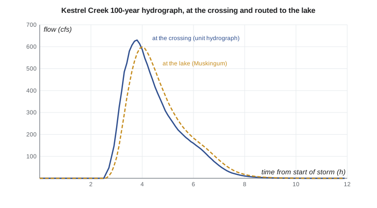
Answer: The peak block alone would produce about 480 cfs at 3.5 hours. The later blocks add their own lagged hydrographs while the first is still near its peak, so the combined flow keeps rising: the convolution of all the blocks, as the script shows, peaks at 638 cfs at 3.8 hours.
Flood routing
A flood changes as it passes through storage. A pond, a lake or a reservoir stores water as the inflow rises and releases it as the inflow falls, so the outflow peak is lower and later than the inflow peak. A channel reach does the same, more mildly. Computing these changes is called flood routing. Hydrologic routing, used here, rests on the continuity equation in the form
where \(S\) is the storage, \(I\) the inflow and \(O\) the outflow, together with a relation between storage and outflow. Hydraulic routing, which solves the full Saint-Venant equations of unsteady flow, is used for large rivers, dam breaks and situations with backwater, and is available in HEC-RAS.
Level-pool routing
For a pond with a horizontal water surface, both the storage and the outflow are functions of the water level alone: the storage from the pond's shape and the outflow from the rating curve of its outlet, as in lesson 6. Writing the continuity equation over a time step \(\Delta t\) with average values gives
The unknowns at the end of the step, \(S_2\) and \(O_2\), both depend on the stage. The storage indication method, also called the modified Puls method, rearranges the equation as \(2S_2/\Delta t + O_2 = I_1 + I_2 + 2S_1/\Delta t - O_1\) and uses a table of \(2S/\Delta t + O\) against stage to solve each step. A small time step with a direct update, as in Sofia's script, gives the same answer. A key property of level-pool routing is that the outflow peak occurs exactly when the outflow hydrograph crosses the falling limb of the inflow hydrograph, the moment when storage is a maximum.
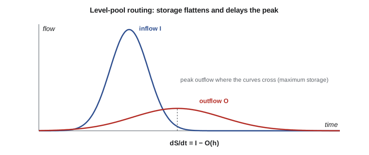
The Kestrel Bay pond has a bottom of 100 ft by 80 ft with side slopes of 4H:1V, so its storage at stage \(h\) is \(S = 8000h + 720h^2 + 21.3h^3\) ft³. Its inflow is the post-development site hydrograph, computed with the same unit hydrograph method in 5-minute blocks, which the short time of concentration requires, and its outflow follows the rating of lesson 6.
Muskingum routing
In a channel reach, storage depends on both inflow and outflow, because the water surface is not level: during the rise, the upstream end is deeper than the downstream end, creating wedge storage. The Muskingum method, developed for the Muskingum River in Ohio in the 1930s, models this as
where \(K\) is about the travel time of the flood wave through the reach and \(X\), between 0 and 0.5, weights the inflow; natural streams typically have \(X\) between 0.1 and 0.3. Combining this with continuity gives the routing equation
with coefficients that sum to 1 and depend on \(K\), \(X\) and \(\Delta t\). To keep all three coefficients positive, the time step should satisfy \(2KX \le \Delta t \le 2K(1 - X)\). The parameters can be calibrated from recorded floods or estimated from the channel geometry; the Muskingum-Cunge variant computes them from the channel properties directly.
Sofia's script builds the creek hydrograph by convolution, builds the site hydrograph and routes it through the pond, and routes the creek flood 1.5 km to the lake with \(K = 0.25\) h and \(X = 0.15\).
# NRCS unit hydrograph for Kestrel Creek, level-pool routing of the site pond, Muskingum routing
from math import sqrt, pi
UNITS = "US"
SI = UNITS == "SI"
# NRCS dimensionless unit hydrograph (t/tp, q/qp)
DUH = [(0, 0), (.2, .1), (.4, .31), (.6, .66), (.8, .93), (1, 1), (1.2, .93), (1.4, .78), (1.6, .56), (1.8, .39),
       (2, .28), (2.4, .147), (2.8, .077), (3.2, .04), (3.6, .021), (4, .011), (4.6, .005), (5, 0)]
def duh(r):
    for (r0, q0), (r1, q1) in zip(DUH, DUH[1:]):
        if r0 <= r <= r1: return q0 + (q1 - q0) * (r - r0) / (r1 - r0)
    return 0.0
def runoff(P, CN):
    S = 25400 / CN - 254; Ia = 0.2 * S
    return 0.0 if P <= Ia else (P - Ia) ** 2 / (P - Ia + S)
storm = [1.4, 1.7, 2.2, 3.0, 5.2, 38.1, 8.8, 3.8, 2.5, 1.9, 1.6, 1.3]   # 6-h 100-year, mm per 30 min (lesson 7)
def excess(CN):
    cum, out, prev = 0.0, [], 0.0
    for p in storm:
        cum += p; q = runoff(cum, CN); out.append(q - prev); prev = q
    return out
def hydrograph(Akm2, tc_h, CN, dt=0.5, step=0.1):
    tp = dt / 2 + 0.6 * tc_h
    qp = 0.208 * Akm2 * 1.0 / tp                 # m3/s per mm of runoff
    ex = excess(CN); n = int(16 / step)
    Q = [0.0] * n
    for k, e in enumerate(ex):
        t0 = k * dt
        for j in range(n):
            t = j * step - t0
            if t > 0: Q[j] += e * qp * duh(t / tp)
    return tp, qp, Q
cf = 1.0 if SI else 35.315                       # m3/s to cfs
uq = "m3/s" if SI else "cfs"
A_creek = 6.4 if SI else 2.5 * 2.59              # km2
tp, qp, Qc = hydrograph(A_creek, 1.25, 75)
pk = max(Qc); tpk = Qc.index(pk) * 0.1
ud, fd = ("mm", 1.0) if SI else ("in.", 25.4)
print(f"Creek: tp = {tp:.2f} h, unit hydrograph peak {qp * cf * fd:.{2 if SI else 0}f} {uq} per {ud} of runoff")
print(f"100-year 6-hour storm, CN 75: peak {pk * cf:.1f} {uq} at {tpk:.1f} h, runoff {sum(excess(75)) / fd:.{1 if SI else 2}f} {ud}")
# site hydrograph after development (5-minute blocks), routed through the dry pond
a_, b_, c_ = 1340.0, 6.0, 0.80
cum = [a_ / (5 * k + b_) ** c_ * 5 * k / 60 for k in range(1, 73)]
inc = [cum[0]] + [cum[k] - cum[k - 1] for k in range(1, 72)]
order = sorted(range(72), key=lambda j: -inc[j]); pos = [35 + ((k + 1) // 2) * (1 if k % 2 else -1) for k in range(72)]
storm = [0.0] * 72
for j, p in zip(order, pos): storm[p] = inc[j]
A_site = 0.075 if SI else 18.5 * 0.004047
tp2, qp2, Qs = hydrograph(A_site, 10 / 60, 89, dt=5 / 60, step=1 / 60)
print(f"Site inflow to pond (5-minute storm blocks): peak {max(Qs) * cf:.2f} {uq}, runoff {sum(excess(89)) / fd:.{1 if SI else 2}f} {ud}")
fm = 1.0 if SI else 0.3048                       # pond and outlet dimensions in m or ft, converted to m
Lb, Wb, zp = (30.0, 25.0, 4.0) if SI else (100.0, 80.0, 4.0)
Lb, Wb = Lb * fm, Wb * fm
d_or, crest, bw, sp, bsp = (0.30, 1.30, 0.6, 1.90, 6.0) if SI else (1.0, 4.25, 2.0, 6.25, 20.0)
d_or, crest, bw, sp, bsp = d_or * fm, crest * fm, bw * fm, sp * fm, bsp * fm
def storage(h): return Lb * Wb * h + zp * (Lb + Wb) * h ** 2 + 4 * zp * zp * h ** 3 / 3
def outflow(h):
    q = 0.0
    if h > d_or / 2: q += 0.62 * pi * d_or ** 2 / 4 * sqrt(2 * 9.81 * (h - d_or / 2))
    if h > crest: q += 1.84 * bw * (h - crest) ** 1.5
    if h > sp: q += 1.70 * bsp * (h - sp) ** 1.5
    return q
step = 60.0; S = 0.0; hmax = 0.0; Omax = 0.0
def stage(Sv):
    lo, hi = 0.0, 4.0
    for _ in range(60):
        m = (lo + hi) / 2
        if storage(m) < Sv: lo = m
        else: hi = m
    return m
for k in range(1, len(Qs)):                      # storage indication with a small time step
    I = (Qs[k - 1] + Qs[k]) / 2
    h = stage(S); O = outflow(h)
    S = max(S + (I - O) * step, 0.0)
    h = stage(S); hmax = max(hmax, h); Omax = max(Omax, outflow(h))
L = "m" if SI else "ft"; fl = 1.0 if SI else 3.2808
print(f"Pond: peak stage {hmax * fl:.2f} {L}, peak outflow {Omax * cf:.2f} {uq}, storage used {storage(hmax) * (1 if SI else 35.315):,.0f} {'m3' if SI else 'ft3'}")
# Muskingum routing of the creek hydrograph through the 1.5 km reach to the lake, K = 0.25 h, X = 0.15, dt = 0.1 h
K, X, d = 0.25, 0.15, 0.1
D = K - K * X + 0.5 * d
c0, c1, c2 = (-K * X + 0.5 * d) / D, (K * X + 0.5 * d) / D, (K - K * X - 0.5 * d) / D
O = [Qc[0]]
for j in range(1, len(Qc)): O.append(c0 * Qc[j] + c1 * Qc[j - 1] + c2 * O[-1])
print(f"Muskingum C0, C1, C2 = {c0:.3f}, {c1:.3f}, {c2:.3f}; outflow peak {max(O) * cf:.1f} {uq} at {O.index(max(O)) * 0.1:.1f} h")Creek: tp = 1.00 h, unit hydrograph peak 1208 cfs per in. of runoff 100-year 6-hour storm, CN 75: peak 637.6 cfs at 3.8 h, runoff 0.84 in. Site inflow to pond (5-minute storm blocks): peak 63.72 cfs, runoff 1.73 in. Pond: peak stage 5.16 ft, peak outflow 14.26 cfs, storage used 63,454 ft3 Muskingum C0, C1, C2 = 0.048, 0.333, 0.619; outflow peak 605.7 cfs at 4.0 h
Reading the results
The creek hydrograph peaks at 638 cfs, 3.8 hours after the storm begins and about an hour after the most intense rain. This is the independent confirmation of the preliminary design flow of 640 cfs used in lessons 2 to 4; lesson 11 adds a second, statistical check. Routing the flood 1.5 km (about a mile) to the lake lowers the peak only slightly, to 606 cfs, and delays it by about 12 minutes; a short, steep reach has little storage.
The pond does much more. The site inflow peaks at 63.7 cfs; the pond rises to 5.16 ft, storing about 63,000 ft³, and releases a peak of only 14.3 cfs, below the pre-development 100-year peak of 15.1 cfs from lesson 9. The design meets the city's quantity control criterion for the 100-year storm. The unit hydrograph inflow peak, 63.7 cfs, is lower than the rational method's 89 cfs, which includes a frequency factor and assumes the whole storm intensity for the time of concentration; the full design report routes both the NRCS hydrograph and a rational-method hydrograph, as reviewers often ask, and repeats the routing for the 2- to 25-year storms to confirm that the orifice alone controls them.
Computer models
In practice, these calculations are done in software. HEC-HMS, from the US Army Corps of Engineers, is free and widely used in both countries; it combines loss methods such as the curve number, transform methods such as the NRCS and Snyder unit hydrographs, and routing methods such as modified Puls and Muskingum-Cunge for networks of subbasins and reaches. The NRCS TR-20 and TR-55 programs, the US Environmental Protection Agency's Storm Water Management Model (SWMM) for urban systems, and commercial packages built on them are also common. Understanding the hand methods is what lets an engineer judge whether a model's output is reasonable.
Practical points
- Choose the time step of the rainfall blocks to suit the time of concentration; about a fifth of \(t_p\) or less.
- Build rainfall excess from cumulative rainfall, not from each block separately.
- Route ponds with the full hydrograph and the actual outlet rating; check several storm durations to find the critical one.
- Keep Muskingum coefficients positive by choosing the time step within the recommended limits.
- Check model results against hand calculations and, where possible, against recorded floods.
Common mistakes
MistakeApplying the curve number equation to each rainfall block separately.
InsteadCompute cumulative runoff, then take increments.
MistakeUsing 30-minute blocks for a site with a 10-minute time of concentration.
InsteadUse blocks short enough to resolve the site's response.
MistakeSizing a pond with the rational method peak only.
InsteadRoute a hydrograph; storage depends on volume and timing.
MistakeChoosing a Muskingum time step smaller than \(2KX\).
Instead\(C_0\) then becomes negative and the routed flow can dip unrealistically.
Summary and key terms
- A unit hydrograph is the runoff from one unit of excess in a given duration; proportionality and superposition give the convolution \(Q_n = \sum P_m U_{n-m+1}\).
- NRCS: \(t_p = D/2 + 0.6t_c\), \(q_p = 0.208A/t_p\) (SI) or \(484A/t_p\) (US).
- Kestrel Creek 100-year peak: 638 cfs at 3.8 h, confirming 640 cfs.
- Level-pool routing: \(dS/dt = I - O\); the outflow peaks where it crosses the inflow.
- Pond: inflow 63.7 cfs, peak stage 5.16 ft, outflow 14.3 cfs ≤ 15.1 cfs allowed.
- Muskingum: \(S = K[XI + (1 - X)O]\), \(O_2 = C_0I_2 + C_1I_1 + C_2O_1\).
- Hydrograph
- A graph of discharge against time at a point on a stream.
- Baseflow
- Streamflow supplied by groundwater between storms.
- Unit hydrograph
- The direct runoff hydrograph from one unit of rainfall excess of a given duration.
- Convolution
- Summing lagged, scaled unit hydrographs to obtain the hydrograph of a complex storm.
- Time to peak
- The time from the start of rainfall excess to the peak of the unit hydrograph.
- Flood routing
- Computing how a flood hydrograph changes as it passes through storage.
- Level-pool routing
- Routing through a reservoir whose storage and outflow depend only on its water level.
- Muskingum method
- A hydrologic channel routing method with storage depending on weighted inflow and outflow.
Practice problems
Work each problem on paper first, then reveal the answer to check.
A 6 mi² watershed has \(t_c = 2.0\) h. With 1-hour blocks, find \(t_p\) and \(q_p\).
Show answer
\(t_p = 0.5 + 1.2 = 1.7\) h; \(q_p = 484(6)/1.7 = 1{,}710\) cfs per in.
A 1-hour unit hydrograph has ordinates 0, 150, 400, 260, 100, 0 cfs per in. at hourly intervals. Two hours of excess of 0.4 in. then 0.8 in. fall. Find the peak flow.
Show answer
Ordinates: 0, 60, 160+120 = 280, 104+320 = 424, 40+208 = 248, 80, 0; peak 424 cfs.
For Muskingum routing with \(K = 2\) h and \(X = 0.2\), what range of time steps keeps all coefficients positive?
Show answer
\(2KX = 0.8\) h to \(2K(1 - X) = 3.2\) h.
Why does the outflow from a level-pool reservoir peak exactly where it meets the falling inflow hydrograph?
Show answer
Storage increases while \(I > O\) and decreases when \(I < O\); maximum storage, and so maximum stage and outflow, occurs when \(I = O\).
Lesson quiz · 5 questions
Score 60% or more to complete this lesson.
Create a free account to save your progress, take quizzes and earn a certificate.