Collecting and interpreting rate data

Every rate law used so far came from someone else: the resin vendor, a textbook or a literature value. Ingrid will not seal a design basis on a vendor's number alone. She asks Dev Raman in the QC lab to measure the esterification rate on the plant's own acetic acid and dry ethanol with a sample of the resin, and asks Theo to analyze the data. This lesson covers how rate data are collected, the classical methods for extracting orders and rate constants from them, the modern method that has largely replaced those, and how the temperature dependence is found.

Laboratory reactors

Rate data come from small reactors designed so that the rate is easy to infer. A batch reactor gives concentration against time, from which the rate must be found by differentiating or by fitting an integrated rate law. A CSTR at steady state gives the rate directly at one composition: \(-r_A = (C_{A0} - C_A)/\tau\), with no differentiation at all, which is why stirred laboratory reactors are popular for catalytic kinetics. A differential packed bed, a short bed run at low conversion, gives the rate at nearly constant composition as \(-r_A' = F_{A0}X/\Delta W\). Lesson 7 uses differential-reactor data for the dehydration catalyst.

Whatever the reactor, the experiment must measure the intrinsic chemical rate and not something else. Two checks are standard. Changing the stirring speed, or the flow velocity past the catalyst, should not change the rate; if it does, mass transfer from the fluid to the catalyst surface is limiting. Changing the particle size should not change the rate; if it does, diffusion inside the particles is limiting. Dev runs both checks first and finds that above 400 rpm the rate no longer depends on stirring and that the crushed and whole resin beads give the same rate at 70 °C, so the data reflect the chemistry.

The method of excess

The esterification rate depends on both acid and ethanol, and on the products through the reverse reaction. Separating these effects in one experiment is hard, so Dev uses a classical trick: a large excess of ethanol, 10 mol per mole of acid, and only the early part of each run, when little product has formed. The ethanol concentration then barely changes, the reverse reaction is negligible, and the rate behaves as \(-r_A = k'C_A^{\alpha}\) with \(k' = kC_B^{\beta}\), a pseudo rate constant. Repeating with a different excess separates \(\beta\) from \(k\). This method of excess, sometimes called isolation, reduces a multi-reactant problem to a single-reactant one.

Three classical analyses

Dev's first run at 70 °C gives the acid concentration at nine times over an hour. Three classical methods extract the order and rate constant.

The differential method estimates the rate at each point by numerical differentiation, then fits \(\ln(-dC_A/dt) = \ln k' + \alpha\ln C_A\). The slope is the order. Differentiation amplifies noise, so the method needs good data and a careful differentiation scheme, such as central differences or a smooth fit through the points.

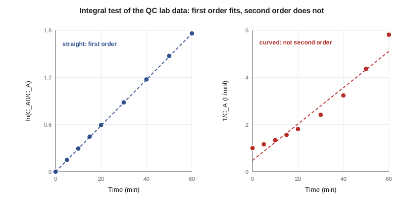
The integral method guesses an order, integrates the rate law, and checks for a straight line. First order predicts that \(\ln(C_{A0}/C_A)\) is linear in time with slope \(k'\); second order predicts that \(1/C_A\) is linear in time. The method averages noise better than differentiation but needs a guess, and two orders can fit almost equally well if the run does not go far enough.

The half-life method uses the time for the concentration to fall by half. For order \(n \ne 1\), \(t_{1/2} = (2^{n-1} - 1)/(k'(n - 1)C_{A0}^{n-1})\); for first order, \(t_{1/2} = \ln 2/k'\), independent of starting concentration. Measuring half-lives at several starting concentrations and plotting \(\ln t_{1/2}\) against \(\ln C_{A0}\) gives a slope of \(1 - n\).

# Analyzing batch rate data from the QC lab: acid-catalyzed esterification with a 10:1 excess of ethanol
# Early in each run the reverse reaction is negligible, so -dCA/dt = k' CA^n with k' a pseudo constant
import math
t = [0, 5, 10, 15, 20, 30, 40, 50, 60]                 # min
CA = [1.000, 0.861, 0.745, 0.640, 0.553, 0.414, 0.309, 0.229, 0.172]   # mol/L acetic acid at 70 C (measured, rounded)

# 1. differential method: central differences, then ln(-dC/dt) against ln C
pts = []
for i in range(1, len(t) - 1):
    r = -(CA[i + 1] - CA[i - 1]) / (t[i + 1] - t[i - 1])
    pts.append((math.log(CA[i]), math.log(r)))
n = len(pts); sx = sum(p[0] for p in pts); sy = sum(p[1] for p in pts)
sxx = sum(p[0] ** 2 for p in pts); sxy = sum(p[0] * p[1] for p in pts)
slope = (n * sxy - sx * sy) / (n * sxx - sx * sx); icpt = (sy - slope * sx) / n
print(f"differential method: order n = {slope:.2f}, k' = {math.exp(icpt):.4f}")

# 2. integral method: first order predicts ln(CA0/CA) linear in t; second order predicts 1/CA linear in t
def fit(xs, ys):
    m = len(xs); mx = sum(xs) / m; my = sum(ys) / m
    b = sum((x - mx) * (y - my) for x, y in zip(xs, ys)) / sum((x - mx) ** 2 for x in xs)
    a = my - b * mx
    ss = sum((y - a - b * x) ** 2 for x, y in zip(xs, ys)); st = sum((y - my) ** 2 for y in ys)
    return b, 1 - ss / st
b1, r1 = fit(t, [math.log(CA[0] / c) for c in CA])
b2, r2 = fit(t, [1 / c for c in CA])
print(f"first order: k' = {b1:.4f} 1/min, R2 = {r1:.5f};  second order: k = {b2:.4f}, R2 = {r2:.5f}")
print(f"half-life from the first-order fit: {math.log(2) / b1:.1f} min")

# 3. nonlinear least squares on C(t) directly, for both k' and n (grid search, then refinement)
def model(kk, nn, tt):
    if abs(nn - 1) < 1e-9: return math.exp(-kk * tt)
    base = 1 + (nn - 1) * kk * tt
    return base ** (1 / (1 - nn)) if base > 0 else 0.0
best = None
for i in range(41):
    nn = 0.6 + i * 0.02
    for j in range(200):
        kk = 0.020 + j * 0.0002
        s = sum((c - model(kk, nn, tt)) ** 2 for c, tt in zip(CA, t))
        if best is None or s < best[0]: best = (s, kk, nn)
print(f"nonlinear fit: k' = {best[1]:.4f}, n = {best[2]:.2f}, sum of squares = {best[0]:.2e}")

# 4. Arrhenius: first-order k' measured at three temperatures
data = [(60, 0.0154), (70, 0.0295), (80, 0.0545)]   # C, 1/min
xs = [1 / (T + 273.15) for T, _ in data]; ys = [math.log(kk) for _, kk in data]
b, _ = fit(xs, ys)
Ea = -b * 8.314 / 1000
print(f"activation energy from the Arrhenius plot: {Ea:.1f} kJ/mol")

differential method: order n = 0.99, k' = 0.0291
first order: k' = 0.0293 1/min, R2 = 0.99998;  second order: k = 0.0771, R2 = 0.94841
half-life from the first-order fit: 23.6 min
nonlinear fit: k' = 0.0298, n = 1.02, sum of squares = 1.18e-05
activation energy from the Arrhenius plot: 61.8 kJ/mol

Reading the results

The differential method gives an order of 0.99 and \(k' = 0.0291\) per minute. The integral test agrees: the first-order plot has \(R^2 = 0.99998\), while the second-order plot curves away with \(R^2 = 0.948\). The half-life is 23.6 minutes. The three methods tell one story: in a large excess of ethanol, the esterification is first order in acetic acid, with a pseudo rate constant of about 0.029 per minute at 70 °C.

Nonlinear regression

The classical methods linearize the rate law so that a straight line can be fitted. Linearizing distorts the errors: taking logarithms, for example, gives small concentrations far more weight than large ones. The modern approach fits the model directly to the measured concentrations by minimizing the sum of squared differences between measured and predicted values,

over the unknown parameters. The code does this with a grid search over \(k'\) and \(n\), a simple method that cannot get lost; practical work uses the Levenberg-Marquardt algorithm, built into every scientific computing package. The fit gives \(k' = 0.0298\) per minute and \(n = 1.02\), confirming first order. Nonlinear regression also gives confidence intervals on the parameters, and the residuals, the differences between data and model, should scatter randomly. A trend in the residuals means the model is wrong, however good the \(R^2\) looks.

Whatever method is used, the fitted parameters are valid only over the range of conditions in the experiments. Dev's runs cover acid concentrations from 1.0 down to 0.17 mol/L in ethanol; the pre-reactor runs at 3 to 8 kmol/m³ of acid with comparable ethanol. Ingrid flags the gap: a rate law fitted in dilute excess ethanol may not hold in the concentrated mixture, where the resin swells differently and water competes for the acid sites. Dev's next series runs at the plant's actual ratio and follows each run to equilibrium, and the reversible rate law is fitted to all the data at once.

Temperature dependence

Repeating the runs at 60, 70 and 80 °C gives three pseudo rate constants: 0.0154, 0.0295 and 0.0545 per minute. The Arrhenius equation in logarithmic form, \(\ln k = \ln A - E/RT\), says that a plot of \(\ln k\) against \(1/T\) is a straight line with slope \(-E/R\).

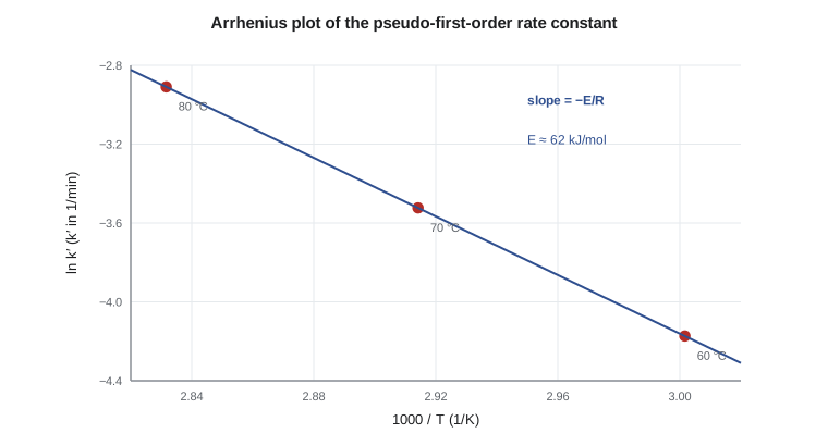
The fit gives an activation energy of 61.8 kJ/mol, in the range typically reported for esterification over acid resins. That number matters for design in two ways. It sets how much the rate rises with temperature, about 85 % for each 10 K here. It also sets how fast the catalyst could run away from its temperature if the reaction released much heat, which for this nearly thermoneutral reaction it does not. Three temperatures is the minimum for an Arrhenius fit; a design-quality measurement would use five or more, spanning the full range of temperatures the reactor will see.

Statistical design of experiments

Dev's experiments vary one factor at a time. A more efficient approach, statistical design of experiments, varies several factors at once in a planned pattern so that their effects and interactions can be separated with fewer runs. For a kinetic study, a factorial design over temperature, acid concentration and ethanol ratio, with a few repeated center points to measure the experimental error, gives more information per run than a one-at-a-time series. The repeated runs also tell the engineer how precise the parameters are, which feeds directly into the design margins of lesson 12.

What the plant can measure

Once the reactor is running, it becomes a source of rate data too. The inlet and outlet compositions, the flow and the bed temperature give an average rate for the whole bed at each set of conditions. Plotting the apparent rate constant from plant data against time on stream shows catalyst aging directly, and comparing it with the laboratory value checks the design basis. Ingrid asks Theo to set up that calculation in the plant historian before start-up, so that the first month of operation confirms or corrects the laboratory kinetics.