Residence time distributions and non-ideal reactors

Every design so far assumed ideal flow, perfect mixing or perfect plug flow. Real vessels are neither. A packed bed has fluid that channels along the wall, eddies behind particles and stagnant pockets; a stirred tank has dead corners and short-circuits from the inlet to the outlet. Before the full-scale pre-reactor is ordered, the resin vendor lends a pilot bed of the same depth and particle size, and Ingrid asks Theo to measure how close it is to plug flow. The tool is a tracer test, and the result is a residence time distribution that tells how long each fluid element spends in the vessel.

The residence time distribution

In an ideal PFR every fluid element spends exactly the space time \(\tau\) in the reactor. In an ideal CSTR, some elements leave almost immediately and others stay much longer; the times are spread out exponentially. Real vessels lie between. The residence time distribution, or RTD, \(E(t)\), is defined so that \(E(t)\,dt\) is the fraction of the fluid leaving the vessel that has spent between \(t\) and \(t + dt\) inside. It is a probability distribution, so its integral over all times is 1. The idea and the methods for measuring it were set out by P. V. Danckwerts in the 1950s, and they remain the standard way to diagnose flow problems in reactors.

Measuring the RTD with a pulse of tracer

A small amount of an inert tracer, a substance that does not react, adsorb or change the flow, is injected quickly at the inlet, and its concentration \(C(t)\) is measured at the outlet. Common tracers are salts measured by conductivity, dyes measured by light absorption, and for some plants radioactive isotopes measured from outside the pipe. For the resin bed, Theo uses lithium chloride at a low concentration, which the acid resin does not exchange appreciably at the test conditions, measured in outlet samples. The RTD is the normalized outlet response,

and two moments describe it. The mean residence time is \(t_m = \int tE(t)\,dt\), which should equal the space time \(\tau = V/v_0\) for a closed vessel with no dead volume; a smaller \(t_m\) means part of the volume is stagnant. The variance \(\sigma^2 = \int (t - t_m)^2E(t)\,dt\) measures the spread. The dimensionless variance \(\sigma^2/t_m^2\) is 0 for plug flow and 1 for a perfect CSTR.

# Residence time distribution of the pilot resin bed from a pulse tracer test, and its effect on conversion
import math
t = [0, 2, 4, 6, 8, 10, 12, 14, 16, 18, 20, 24, 28, 32, 36, 40]           # min
C = [0, 0.05, 0.60, 2.10, 3.90, 4.80, 4.70, 3.90, 2.90, 2.00, 1.30, 0.50, 0.18, 0.06, 0.02, 0.0]   # mg/L lithium tracer (measured, rounded)
def trap(y, x): return sum((x[i + 1] - x[i]) * (y[i] + y[i + 1]) / 2 for i in range(len(x) - 1))
area = trap(C, t)
E = [c / area for c in C]
tm = trap([ti * e for ti, e in zip(t, E)], t)
var = trap([(ti - tm) ** 2 * e for ti, e in zip(t, E)], t)
N = tm ** 2 / var
print(f"tracer area {area:.2f} mg min/L, mean residence time {tm:.1f} min, variance {var:.1f} min2")
print(f"tanks-in-series number N = {N:.1f}; dimensionless variance {var / tm ** 2:.3f}")
# open-open dispersion: sigma2 = 2/Pe + 8/Pe^2, solve for Pe
lo, hi = 0.5, 500.0
for _ in range(100):
    Pe = (lo + hi) / 2
    f = 2 / Pe + 8 / Pe ** 2 - var / tm ** 2
    lo, hi = (Pe, hi) if f > 0 else (lo, Pe)
print(f"dispersion model: Peclet number about {Pe:.1f}")

# conversion of the reversible esterification (lesson 2 kinetics) with this RTD
K, kc = 4.0, 1.5e-4 * 8.7 * 60       # kc = k CA0 in 1/min
def batch_X(tt, h=0.05):
    X = 0.0; s = 0.0
    while s < tt - 1e-9:
        f = lambda X: kc * ((1 - X) ** 2 - X ** 2 / K)
        a = f(X); b = f(X + h * a / 2); c = f(X + h * b / 2); d = f(X + h * c)
        X += h * (a + 2 * b + 2 * c + d) / 6; s += h
    return X
X_pfr = batch_X(tm)
# segregation model: average the batch conversion over the measured E(t)
X_seg = trap([batch_X(ti) * e for ti, e in zip(t, E)], t) / trap(E, t)
# tanks in series (rounded N), each CSTR solved for X by bisection
def cstr_series(n, tau_total):
    X = 0.0; ti = tau_total / n
    for _ in range(n):
        lo, hi = X, 2 / 3
        for _ in range(60):
            m = (lo + hi) / 2
            if m - X - ti * kc * ((1 - m) ** 2 - m ** 2 / K) < 0: lo = m
            else: hi = m
        X = m
    return X
n = round(N)
print(f"ideal PFR at tm: X = {X_pfr:.3f}; segregation model: X = {X_seg:.3f}; {n} tanks in series: X = {cstr_series(n, tm):.3f}; one CSTR: X = {cstr_series(1, tm):.3f}")
print(f"equilibrium limit 0.667; the measured bed loses {100 * (X_pfr - cstr_series(n, tm)) / X_pfr:.1f} % of the ideal conversion")

tracer area 56.84 mg min/L, mean residence time 12.9 min, variance 26.2 min2
tanks-in-series number N = 6.3; dimensionless variance 0.158
dispersion model: Peclet number about 15.9
ideal PFR at tm: X = 0.482; segregation model: X = 0.462; 6 tanks in series: X = 0.457; one CSTR: X = 0.368
equilibrium limit 0.667; the measured bed loses 5.4 % of the ideal conversion

Reading the tracer test

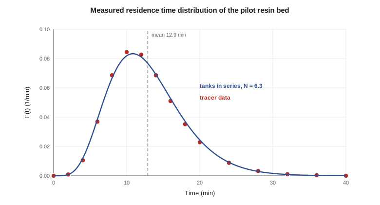
The tracer comes out between about 2 and 36 minutes, peaking near 11 minutes, with a mean residence time of 12.9 minutes. The pilot bed's space time, from its volume and the test flow, is 13 minutes, so the mean matches: there is no significant dead volume or bypass. The variance is 26 min², a dimensionless variance of 0.158: the flow is closer to plug flow than to a CSTR, but not ideal. A real bed always shows some spread, from velocity differences between the center and the wall, from mixing as fluid splits and rejoins around particles, and from diffusion into and out of the resin beads.

Models of non-ideal flow

Two one-parameter models turn the variance into a description that can be used in design. The tanks-in-series model represents the vessel as \(N\) equal CSTRs in series; its RTD has dimensionless variance \(1/N\), so \(N = t_m^2/\sigma^2\). The pilot bed gives \(N = 6.3\). The dispersion model represents the vessel as a PFR with a superimposed axial mixing, characterized by a Peclet number, the ratio of transport by flow to transport by dispersion. For a vessel with open boundaries, \(\sigma^2/t_m^2 = 2/Pe + 8/Pe^2\), which gives \(Pe\) of about 16. Both models fit the measured curve similarly here; the tanks-in-series model is easier to compute with, and the dispersion model connects to correlations for dispersion in packed beds that can be used to scale the result to the full-size bed.

From RTD to conversion

For a first-order reaction, the RTD alone predicts conversion exactly, because each fluid element converts according to how long it stays, independent of what it mixes with. The mean conversion is the batch conversion averaged over the RTD:

This is the segregation model, which treats the flow as many small packets that never mix with each other. For other orders, the RTD is not enough on its own: when fluid elements of different ages mix also matters. The segregation model gives one limit, and the model of maximum mixedness, in which fluid mixes as early as the RTD allows, gives the other. For reactions of order greater than one, segregation gives the higher conversion; for order less than one, maximum mixedness does. The true answer lies between, and for a packed bed with modest dispersion the two limits are close.

For the esterification, Theo computes three predictions at the measured mean residence time of 12.9 minutes, using the reversible rate law of lesson 2. An ideal PFR would give 48.2 %. The segregation model, averaging the batch conversion over the measured RTD, gives 46.2 %. Six tanks in series give 45.7 %. A single CSTR would give only 36.8 %. The pilot bed therefore loses about 5 % of the conversion an ideal plug-flow bed would reach, a gap Theo can cover in the full-scale design with about 10 % more bed volume. Lesson 12 carries that margin into the design.

Diagnosing flow problems

RTDs are also a troubleshooting tool. A sharp early peak means bypassing: some fluid short-circuits from inlet to outlet without contacting most of the bed, as happens when a liquid distributor is blocked or a bed has settled and left a gap at the wall. A long tail means stagnant zones that exchange slowly with the main flow. A mean residence time well below the space time means dead volume, part of the vessel that the flow does not reach. Several peaks can mean parallel paths of different lengths. Each pattern points to a different repair, and a tracer test before and after maintenance confirms that the repair worked. Plants with large catalytic beds sometimes run tracer tests during start-up to check the loading of the catalyst.

In stirred tanks, a tracer test checks the mixing. A good mixer gives an RTD close to the exponential of an ideal CSTR; dead corners show as a long tail, and an inlet placed too near the outlet shows as an early spike. Fermenters, wastewater basins and chlorine contact tanks are routinely tested this way; in water treatment, the measured RTD sets the disinfection credit a contact tank can claim, which links reaction engineering directly to public health regulation.

Beyond one-parameter models

When a one-parameter model does not fit, engineers combine ideal elements: a CSTR in series with a PFR, a main flow with a bypass stream, an active zone exchanging with a dead zone. The parameters are chosen to match the measured RTD and then used to predict conversion. For complex geometries, computational fluid dynamics can predict the flow field and the RTD before a vessel is built, and is increasingly used to design distributors and internals. The tracer test remains the check on the real equipment.