
BIOL-430 · Lesson 9 of 12 · 25 min
Animal movement and telemetry
Where animals go, how far and why are questions that counts and plots cannot answer. Telemetry, tracking individual animals with devices that report their locations, has turned movement into one of the most data-rich parts of ecology. A single GPS collar can record thousands of locations a year, revealing home ranges, habitat choices, migration routes, responses to roads and fences, and the timing of births and deaths. In the running study, the team fits GPS collars to six white-tailed deer that use the wetlands and groves, to learn whether deer use fenced wetland margins differently after cattle are removed. This lesson covers tracking technologies, data quality, home range estimation, habitat selection and the analysis of movement paths.
Tracking technologies
VHF radio telemetry, developed in the 1960s, fits animals with a transmitter that emits pulses on a unique frequency. A researcher with a directional antenna locates the animal by homing in on it or by triangulating bearings from two or more known positions. VHF tags are small, light and long-lived, so they remain the only option for many small animals such as bats, songbirds and snakes, but each location takes time and effort and triangulation error can be tens of meters or more.
GPS tags calculate their own position from satellite signals at programmed intervals and either store the locations for later download or send them through cellular networks or satellite systems such as Iridium or Argos. Fix rates of one location every few minutes to every few hours are common. GPS tags are heavier and need more power than VHF tags, so they are used mainly on larger animals, although tags small enough for some songbirds now exist. Other approaches include light-level geolocators, which estimate latitude and longitude from day length and the timing of solar noon with errors of about 100 to 200 kilometers, adequate for long migrations; automated radio telemetry networks, such as the Motus Wildlife Tracking System, run by Birds Canada with partners across the Americas, in which tiny tags are detected by a network of receiving towers; and accelerometers and other sensors that record behavior, heart rate or temperature.
| Technology | Typical tag mass | Location accuracy | Best for |
|---|---|---|---|
| VHF radio | 0.2 g and up | Tens to hundreds of meters by triangulation | Small animals, local movements, survival studies |
| GPS with store-on-board or remote download | 10 g to over 500 g | Usually under 10 to 30 m | Large mammals, raptors, waterfowl |
| Argos satellite | 2 g and up | Hundreds of meters to kilometers | Marine and long-distance migrants |
| Light-level geolocator | Under 1 g | 100 to 200 km | Migratory songbirds; tags must be recovered |
| Automated radio network (Motus) | 0.2 g and up | Detection within range of towers | Migration and stopover of small birds, bats, insects |
Capture, tagging and welfare
Tagging begins with capture, which carries risk for animals and people. White-tailed deer are typically captured with drop nets, box traps or chemical immobilization by darting, under a wildlife agency permit and an approved animal care protocol, often with a veterinarian. Collars must fit properly, allowing for neck swelling in the rut, and should include a release mechanism or a planned recapture so that animals do not carry them indefinitely. Tag mass should stay below welfare guidelines, often 3 to 5 percent of body mass for mammals and less for birds. Tags can change behavior, survival or reproduction, and studies should check for such effects, for example by comparing tagged and untagged animals where possible.
Location data quality
GPS locations are not perfect. Fix success, the fraction of scheduled attempts that produce a location, drops under dense canopy and in steep terrain, so habitats such as dense aspen groves may be underrepresented in the data, a habitat-induced bias. Location error varies with the number of satellites and their geometry, summarized by the dilution of precision (DOP) value stored with each fix. Standard screening removes fixes with high DOP, two-dimensional fixes with few satellites, and implausible locations that imply impossible movement speeds. Collars should be tested at known locations in different habitats before deployment to measure fix success and error.
Home ranges
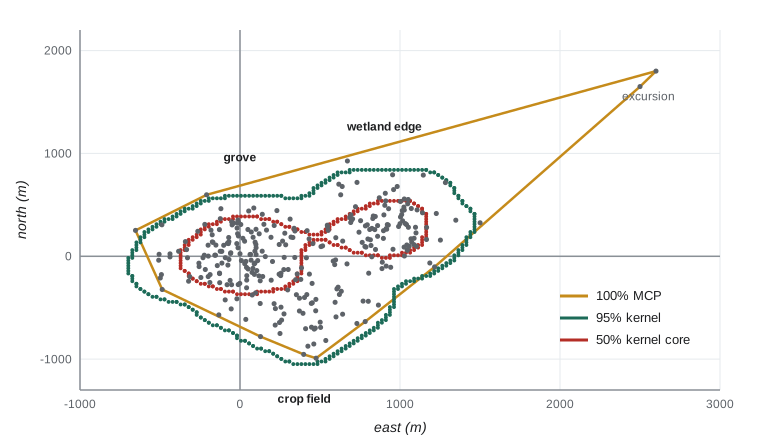
Burt defined the home range in 1943 as the area traversed by an individual in its normal activities of food gathering, mating and caring for young. Estimating it from locations requires choices. The minimum convex polygon (MCP) connects the outermost locations into the smallest convex shape. It is simple and comparable with older studies but sensitive to outliers and sample size, and it includes unused areas inside the polygon. Excluding the outermost 5 percent of points, giving a 95 percent MCP, reduces sensitivity to occasional excursions.
Kernel density estimation (KDE) places a smooth bump, the kernel, over each location and sums them to produce a utilization distribution, the probability density of the animal's location. The home range is the smallest area containing a stated fraction of that density, usually 95 percent, and the core area is often the 50 percent contour. The result depends strongly on the bandwidth, the width of each kernel: too narrow fragments the range into islands around points; too wide inflates it. Reference bandwidths, least-squares cross-validation and plug-in methods are common choices, each with known biases. Because GPS locations taken minutes apart are strongly autocorrelated, methods designed for independent points underestimate ranges; autocorrelated KDE (AKDE), developed by Fleming and colleagues in 2015, models the autocorrelation explicitly and is increasingly standard.
# Home range of a collared deer: minimum convex polygon versus kernel density (synthetic GPS fixes).
import numpy as np
from scipy.spatial import ConvexHull
from scipy.stats import gaussian_kde
rng = np.random.default_rng(909)
hubs = np.array([[0, 0], [900, 300], [400, -500]])       # m: grove, wetland edge, crop field
weights = [0.5, 0.35, 0.15]
k = rng.choice(3, 600, p=weights)
xy = hubs[k] + rng.normal(0, 220, (600, 2))
xy = np.vstack([xy, [[2600, 1800], [2500, 1650]]])          # a two-fix excursion
mcp100 = ConvexHull(xy).volume / 1e6
d = np.hypot(*(xy - xy.mean(0)).T)
keep = xy[d <= np.quantile(d, 0.95)]
mcp95 = ConvexHull(keep).volume / 1e6
kde = gaussian_kde(xy.T)
gx, gy = np.meshgrid(np.linspace(-1200, 3000, 260), np.linspace(-1600, 2400, 260))
dens = kde(np.vstack([gx.ravel(), gy.ravel()]))
cell = (4200 / 259) * (4000 / 259) / 1e6
order = np.sort(dens)[::-1]; cum = np.cumsum(order) * cell
for level in (0.95, 0.50):
    thr = order[np.searchsorted(cum / cum[-1], level)]
    print(f"KDE {int(level * 100)}% area: {np.sum(dens >= thr) * cell:.2f} km2")
print(f"MCP 100%: {mcp100:.2f} km2, MCP 95%: {mcp95:.2f} km2 (the excursion inflates the 100% polygon)")KDE 95% area: 2.61 km2 KDE 50% area: 0.69 km2 MCP 100%: 3.92 km2, MCP 95%: 2.22 km2 (the excursion inflates the 100% polygon)
The two excursion fixes nearly double the full polygon compared with the 95 percent polygon. The kernel results show both strengths and a weakness of the method: the 50 percent core, about 0.7 square kilometers, picks out the grove and wetland edge where the deer spends most of its time, but the 95 percent contour is larger than the 95 percent polygon, because the default reference bandwidth, designed for a single bell-shaped cluster, oversmooths a range with three separate centers of activity. A smaller bandwidth chosen by cross-validation, or an autocorrelated kernel method, would tighten it. Reporting the method and bandwidth is therefore as important as reporting the area.
Habitat selection
Use of a habitat means little on its own; a deer may spend most of its time in cropland simply because cropland covers most of the landscape. Selection compares use with availability. Johnson (1980) described orders of selection: first order, the geographic range of a species; second order, the placement of a home range within the landscape; third order, the use of habitats within the home range; and fourth order, the choice of particular food items or sites within a habitat patch. Conclusions can differ between orders, so studies must state which they address.
Resource selection functions (RSFs) model the relative probability of use as a function of habitat covariates. In a used-available design, each GPS location is compared with a set of random points from the area considered available, such as the home range, and logistic regression estimates coefficients \(\beta\); the RSF is \(w(x) = \exp(\beta_1 x_1 + \beta_2 x_2 + \dots)\), proportional to the probability of selection. A positive coefficient for distance to water, for instance, would mean avoidance of water. Step selection functions refine this by comparing each observed step with alternative steps the animal could have taken from the same starting point, which matches availability to what is actually reachable and accounts for movement constraints.
# Resource selection function: used GPS fixes vs available random points (synthetic covariates).
import numpy as np
from scipy.optimize import minimize
rng = np.random.default_rng(80)
n_av = 3000
dist_edge = rng.uniform(0, 600, n_av)            # m from wetland edge
grove = rng.uniform(size=n_av) < 0.25            # inside aspen grove
fenced = rng.uniform(size=n_av) < 0.20           # inside a fenced margin
beta_true = np.array([-0.004, 1.2, 0.6])
X_av = np.column_stack([dist_edge, grove, fenced]).astype(float)
w = np.exp(X_av @ beta_true)
used = X_av[rng.choice(n_av, 800, p=w / w.sum())]
X = np.vstack([used, X_av]); y = np.r_[np.ones(len(used)), np.zeros(n_av)]
Xs = np.column_stack([np.ones(len(X)), X[:, 0] / 100, X[:, 1], X[:, 2]])
def nll(b):
    eta = Xs @ b
    return np.sum(np.logaddexp(0, eta)) - y @ eta
b = minimize(nll, np.zeros(4), method='BFGS').x
print(f"distance to wetland edge (per 100 m): {b[1]:+.2f}  -> RSF ratio {np.exp(b[1]):.2f} per 100 m")
print(f"aspen grove: {b[2]:+.2f} -> {np.exp(b[2]):.1f} times relative selection")
print(f"fenced margin: {b[3]:+.2f} -> {np.exp(b[3]):.1f} times relative selection")distance to wetland edge (per 100 m): -0.39 -> RSF ratio 0.68 per 100 m aspen grove: +1.15 -> 3.2 times relative selection fenced margin: +0.65 -> 1.9 times relative selection
The intercept of a used-available logistic regression has no meaning, because the ratio of used to available points is set by the researcher; only the slopes, and their exponentials as relative selection strengths, are interpreted. Defining availability is the crucial decision: the same data can show selection or avoidance depending on whether availability is the home range or the whole study area.
Movement paths
A sequence of GPS fixes is a path that can be broken into steps, the straight-line distance between successive fixes, and turning angles, the change in direction between steps. Step-length and turning-angle distributions differ among behaviors: foraging animals make short, tortuous steps, traveling animals long, straight ones. Hidden Markov models, now widely used in movement ecology, treat these behavioral states as hidden and estimate them, and the probabilities of switching between them, from the observed steps and angles. Net squared displacement, the squared distance from the starting point over time, separates residents from migrants and dispersers. Nathan and colleagues' movement ecology paradigm (2008) frames all of this around the animal's internal state, its motion and navigation capacities, and external factors.
# Step lengths and turning angles reveal resting, foraging and travelling (synthetic 2-hour fixes).
import numpy as np
rng = np.random.default_rng(42)
states = np.repeat([0, 1, 2, 1, 0], [20, 30, 10, 30, 20])   # rest, forage, travel
mean_step = np.array([20, 120, 600]); conc = np.array([0.3, 0.8, 6.0])
heading, xy = 0.0, [np.zeros(2)]
steps, turns = [], []
for s in states:
    turn = rng.vonmises(0, conc[s]); heading += turn
    L = rng.gamma(2, mean_step[s] / 2)
    xy.append(xy[-1] + L * np.array([np.cos(heading), np.sin(heading)]))
    steps.append(L); turns.append(turn)
steps, turns = np.array(steps), np.array(turns)
for s, name in enumerate(['resting', 'foraging', 'travelling']):
    m = states == s
    print(f"{name:10s}: median step {np.median(steps[m]):5.0f} m, mean |turn| {np.degrees(np.abs(turns[m])).mean():5.1f} deg")
nsd = np.sum((np.array(xy) - xy[0]) ** 2, axis=1)
print(f"net squared displacement after 110 fixes: {nsd[-1] / 1e6:.2f} km2")resting : median step 15 m, mean |turn| 74.0 deg foraging : median step 87 m, mean |turn| 66.1 deg traveling: median step 454 m, mean |turn| 25.8 deg net squared displacement after 110 fixes: 39.59 km2
Sharing and protecting movement data
Movebank, hosted by the Max Planck Institute of Animal Behavior, stores and shares billions of animal locations from thousands of studies, with controls that let owners restrict access. Location data for vulnerable species can be misused, for example by poachers or by people seeking to disturb animals, so data from species at risk, and locations of dens, nests and roosts, are often generalized or withheld. Indigenous and landowner partners may also have views on how location data from their lands are shared, which should be settled in data agreements before collection begins, as lesson 3 described.
Worked problem
Interpreting an RSF coefficient
A step selection analysis gives a coefficient of 0.69 for fenced margins (yes or no) and -0.35 per 100 m for distance to the nearest grove. Interpret both.
Show solution
- exp(0.69) = 2.0: a step ending in a fenced margin is about twice as likely to be chosen as an otherwise identical step ending outside one.
- exp(-0.35) = 0.70: each additional 100 m from a grove multiplies relative selection by 0.7, so deer prefer locations near groves.
- Because the design is used versus available, these are relative selection strengths, not absolute probabilities of use.
Answer: Fenced margins are selected about twice as strongly, and relative selection falls by about 30 percent for every 100 m away from groves.
Common mistakes
MistakeReporting 100 percent MCP areas as the home range without caveats.
InsteadReport sample sizes, use 95 percent or kernel estimates and consider autocorrelated methods.
MistakeTreating habitat use as habitat selection.
InsteadCompare use with availability and state the order of selection.
MistakeInterpreting the intercept of a used-available model.
InsteadInterpret only slopes as relative selection strengths.
MistakeIgnoring fix success and location error.
InsteadTest collars in each habitat, screen poor fixes and consider habitat-induced bias.
MistakePublishing exact locations of sensitive sites.
InsteadGeneralize or restrict access to sensitive location data.
Summary and key terms
- VHF, GPS, satellite, geolocator and automated networks trade tag mass against accuracy and data volume.
- Capture and tagging require permits, animal care approval and attention to tag mass and fit.
- GPS data need screening for location error and awareness of habitat-related fix failure.
- Home ranges are estimated by MCP or kernel methods; bandwidth and autocorrelation matter.
- Resource and step selection functions compare used locations with available ones to estimate relative selection.
- Step lengths and turning angles reveal behavioral states; movement data must be shared responsibly.
- VHF telemetry
- Locating animals by radio transmitters and directional antennas.
- fix success
- The proportion of scheduled GPS location attempts that succeed.
- dilution of precision
- An index of GPS location quality based on satellite geometry.
- home range
- The area traversed by an animal in its normal activities.
- minimum convex polygon
- The smallest convex polygon containing an animal's locations.
- utilization distribution
- The probability density of an animal's location in space.
- bandwidth
- The width of the kernel used in kernel density estimation.
- resource selection function
- A function proportional to the probability of selecting a resource unit given its covariates.
- step selection function
- A model comparing observed movement steps with available alternative steps.
- turning angle
- The change in direction between successive movement steps.
Practice problems
Work each problem on paper first, then reveal the answer to check.
Why might dense aspen groves be underrepresented in GPS data?
Show answer
Canopy reduces fix success, so locations there fail more often.
A deer weighs 55 kg. What is the maximum collar mass under a 3 percent guideline?
Show answer
1.65 kg.
What happens to a kernel home range if the bandwidth is too wide?
Show answer
It becomes oversmoothed and too large.
Define third-order selection.
Show answer
Selection of habitats within the home range.
An RSF coefficient is -0.5 for road density. What is the relative selection ratio for a one-unit increase?
Show answer
exp(-0.5) = 0.61.
Why are steps of a traveling animal long and straight?
Show answer
Directed movement between areas involves large displacements and small turns.
What is Motus?
Show answer
An automated radio telemetry network of receiving towers that detect small tags.
Why should exact den locations of a species at risk not be published?
Show answer
They could be used to disturb or harm the animals.
Lesson quiz · 5 questions
Score 60% or more to complete this lesson.
Create a free account to save your progress, take quizzes and earn a certificate.