
BIOL-430 · Lesson 10 of 12 · 26 min
Spatial ecology, GIS and remote sensing
Everything in ecology happens somewhere, and where it happens matters. Nearby wetlands share weather, soils and colonists, so they tend to resemble each other; animals respond to the landscape around a site, not just the site itself; and satellites now measure vegetation over whole regions every few days. This lesson covers the tools that make space part of field ecology: spatial autocorrelation and how to measure it, scale and landscape metrics, the basics of geographic information systems and coordinate systems, remote sensing of vegetation, and species distribution models. Lesson 1 introduced grain and extent; here we put numbers to them.
Spatial autocorrelation
Tobler's first law of geography says that everything is related to everything else, but near things are more related than distant things. In ecology, this positive spatial autocorrelation arises because environmental drivers such as soil moisture are themselves spatially structured, and because processes such as dispersal, clonal growth and social attraction link nearby places. Autocorrelation is information, since its scale reveals the scale of the processes that create it, and it is also a statistical problem, because nearby samples are not independent. Treating them as independent overstates the effective sample size, which narrows confidence intervals and inflates false positives, in the same way as the pseudoreplication of lesson 2.
Moran's I measures autocorrelation for a variable \(x\) measured at \(n\) locations, with spatial weights \(w_{ij}\) that are large for neighboring locations:
Values near \(-1/(n-1)\), close to zero, indicate no autocorrelation; positive values mean similar values cluster; negative values mean neighbors tend to differ, as in a checkerboard. A permutation test, shuffling values among locations and recomputing I many times, gives a p-value. Computing I for successive distance classes produces a correlogram, showing over what distances similarity persists.
# Moran's I for vegetation height on a 20 x 20 grid of quadrats: autocorrelated vs random patterns.
import numpy as np
rng = np.random.default_rng(13)
n = 20
def smooth_field(scale):
    z = rng.normal(size=(n + 10, n + 10))
    k = np.exp(-np.add.outer(np.arange(-5, 6)**2, np.arange(-5, 6)**2) / (2 * scale**2))
    out = np.zeros((n, n))
    for i in range(n):
        for j in range(n):
            out[i, j] = np.sum(z[i:i + 11, j:j + 11] * k)
    return (out - out.mean()) / out.std()
def morans_i(x):
    v = x - x.mean(); num = 0.0; W = 0
    for di, dj in [(0, 1), (1, 0)]:                       # rook adjacency, each pair counted twice
        a = v[:n - di, :n - dj]; b = v[di:, dj:]
        num += 2 * np.sum(a * b); W += 2 * a.size
    return (x.size / W) * num / np.sum(v**2)
for name, x in [('patchy (moisture-driven)', smooth_field(1.2)), ('random', rng.normal(size=(n, n)))]:
    I = morans_i(x)
    perm = [morans_i(rng.permutation(x.ravel()).reshape(n, n)) for _ in range(499)]
    p = (1 + np.sum(np.array(perm) >= I)) / 500
print(f"{name:26s} Moran's I = {I:+.3f}, permutation p = {p:.3f}")patchy (moisture-driven) Moran's I = +0.875, permutation p = 0.002 random Moran's I = +0.003, permutation p = 0.474
Semivariograms
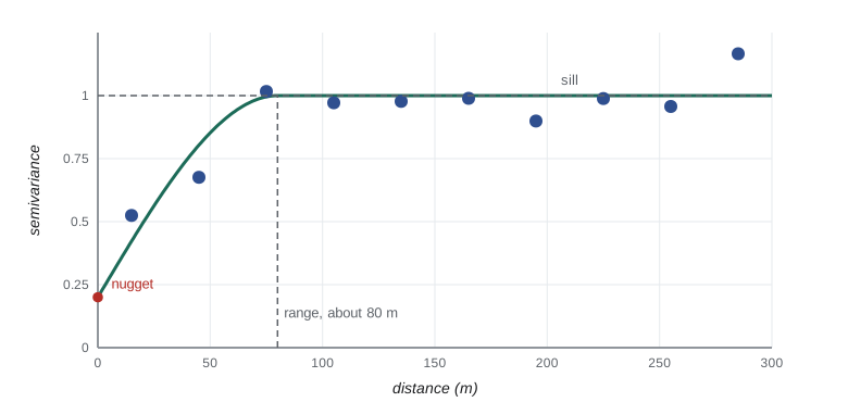
Geostatistics describes spatial structure with the semivariogram, the average half squared difference between values at pairs of locations separated by distance \(h\): \(\gamma(h) = \frac{1}{2N(h)} \sum (x_i - x_j)^2\), summed over the \(N(h)\) pairs in each distance class. For autocorrelated data, the semivariance rises with distance and levels off. The distance at which it levels off is the range, beyond which observations are effectively independent; the plateau is the sill; and the intercept at zero distance, the nugget, represents measurement error and variation at scales finer than the sampling interval. Fitted semivariogram models underpin kriging, which interpolates values between sample points, for example to map soil moisture across a pasture from probe readings.
# Empirical semivariogram of soil moisture probe readings across a pasture (synthetic).
import numpy as np
rng = np.random.default_rng(67)
pts = rng.uniform(0, 400, (150, 2))
d = np.hypot(*(pts[:, None, :] - pts[None, :, :]).transpose(2, 0, 1))
cov = 0.8 * np.exp(-d / 40.0) + 0.2 * np.eye(len(pts))    # exponential model, scale 40 m, nugget 0.2
z = np.linalg.cholesky(cov + 1e-9 * np.eye(len(pts))) @ rng.normal(size=len(pts))
iu = np.triu_indices(len(pts), 1)
dd, sq = d[iu], 0.5 * (z[iu[0]] - z[iu[1]])**2
for lo in range(0, 300, 30):
    m = (dd >= lo) & (dd < lo + 30)
print(f"{lo:3d}-{lo + 30:3d} m: pairs {m.sum():4d}, semivariance {sq[m].mean():.2f}")0- 30 m: pairs 174, semivariance 0.64 30- 60 m: pairs 523, semivariance 0.87 60- 90 m: pairs 781, semivariance 1.00 90-120 m: pairs 950, semivariance 1.00 120-150 m: pairs 1092, semivariance 1.01 150-180 m: pairs 1154, semivariance 1.08 180-210 m: pairs 1199, semivariance 1.06 210-240 m: pairs 1165, semivariance 1.02 240-270 m: pairs 1095, semivariance 1.03 270-300 m: pairs 978, semivariance 0.97
In this synthetic pasture, semivariance climbs from about 0.6 in the closest distance class to a sill near 1.0 by 60 to 90 meters and then stays flat, so readings more than about 80 meters apart are effectively independent. The value in the first class is well above zero partly because of the nugget of measurement error built into the simulation.
Practical consequences follow. Samples spaced closer than the range are partly redundant; analyses of autocorrelated data should include spatial structure, for example through spatial random effects, generalized least squares with a spatial correlation structure, or block cross-validation of predictive models; and the range itself is an ecological result, telling you the scale of patchiness that processes such as grazing or groundwater create.
Scale and landscape metrics
Landscape ecology studies how the composition and configuration of habitat patches affect ecological processes. Composition describes how much of each land cover type there is; configuration describes how it is arranged. Metrics calculated from land cover maps, made popular by the FRAGSTATS software of McGarigal and Marks, include the number and density of patches, mean patch size, edge density, the proportion of the landscape in each class, shape indices, nearest-neighbor distances between patches and connectivity. Many metrics are correlated with each other and with the proportion of habitat, so a few well-chosen ones are better than dozens.
Landscape metrics depend on scale. The same map at 1-meter grain shows individual shrubs and small wetlands that disappear at 30-meter grain; extent determines whether rare land covers are included at all. Ecological responses also have characteristic scales of effect: grassland bird abundance may respond to the amount of grassland within 400 meters, amphibian occupancy to wetland density within a kilometer, and duck nest success to the amount of cropland within several kilometers. Multiscale analyses, which test the same metric in buffers of increasing size around each site and choose the scale with the strongest relationship, have become standard, although they risk overfitting when many scales are tried.
# Landscape metrics from a small land cover raster: patches, edge density and habitat proportion.
import numpy as np
from scipy import ndimage
rng = np.random.default_rng(2)
z = ndimage.gaussian_filter(rng.normal(size=(120, 120)), 6)
grass = (z > np.quantile(z, 0.62)) | (rng.uniform(size=z.shape) < 0.03)   # grassland plus small remnants, 30 m cells
def metrics(mask, cell):
    lab, k = ndimage.label(mask)
    sizes = ndimage.sum(mask, lab, range(1, k + 1)) * cell**2 / 1e4
    edges = np.sum(mask[:, 1:] != mask[:, :-1]) + np.sum(mask[1:, :] != mask[:-1, :])
    area_ha = mask.size * cell**2 / 1e4
    return k, sizes.mean(), edges * cell / area_ha, mask.mean()
for cell, m in [(30, grass), (90, grass.reshape(40, 3, 40, 3).mean((1, 3)) > 0.5)]:
    k, ms, ed, pland = metrics(m, cell)
print(f"{cell} m grain: {k:3d} patches, mean patch {ms:6.1f} ha, edge density {ed:5.1f} m/ha, grassland {pland:.0%}")30 m grain: 222 patches, mean patch 2.3 ha, edge density 41.3 m/ha, grassland 40% 90 m grain: 6 patches, mean patch 83.0 ha, edge density 20.6 m/ha, grassland 38%
GIS and coordinate systems
A geographic information system stores, analyses and maps spatial data. Vector data represent features as points (plot centers, GPS fixes), lines (transects, roads, streams) and polygons (wetlands, pastures); raster data represent continuous surfaces or classified maps as grids of cells (elevation, land cover, satellite images). Common operations include buffering, overlay and intersection, zonal statistics, distance calculations and terrain analysis from digital elevation models, such as the topographic wetness index, which predicts where water accumulates. Free software such as QGIS and the spatial packages of R and Python make these tools widely available.
Every coordinate means something only with its coordinate reference system. Latitude and longitude are angles on an ellipsoid defined by a datum; projected systems such as Universal Transverse Mercator (UTM) convert them to meters on a flat grid within zones 6 degrees of longitude wide. Mixing datums or projections, for example plotting GPS points recorded in WGS 84 on a map in a different datum or zone, can shift locations by meters to hundreds of meters. Field crews should record the datum and coordinate system with every location, set GPS units consistently and check new data against a base map.
The Minnesota study area lies in UTM zone 15, and United States federal and state data commonly use the NAD83 datum, with a modernized national datum in development by the National Geodetic Survey. Free base data include USGS topographic maps and 3DEP elevation data and the National Wetlands Inventory from the U.S. Fish and Wildlife Service.
Remote sensing of vegetation
Satellites and aircraft measure reflected light in several wavelength bands. Healthy green vegetation absorbs red light for photosynthesis and strongly reflects near-infrared light because of leaf cell structure, so the normalized difference vegetation index, \(NDVI = (NIR - Red)/(NIR + Red)\), ranges from near zero or negative for water, bare soil and snow to about 0.8 or more for dense green vegetation. Time series of NDVI track green-up, senescence, drought and grazing. The Landsat program has imaged the Earth at 30-meter resolution since 1972, with Landsat 8 and 9 now in orbit, and the European Copernicus Sentinel-2 satellites provide 10-meter imagery in the visible and near-infrared every few days, both free. Drones carrying multispectral cameras give centimeter resolution over small areas, and airborne lidar measures vegetation height and structure in three dimensions.
# NDVI from synthetic Sentinel-2 red (B4) and near-infrared (B8) reflectance for a pasture and wetlands.
import numpy as np
rng = np.random.default_rng(208)
H = W = 60                                    # 60 x 60 cells of 10 m (600 m square)
yy, xx = np.mgrid[0:H, 0:W]
water = (xx - 18)**2 + (yy - 20)**2 < 60
wet_edge = ((xx - 18)**2 + (yy - 20)**2 < 160) & ~water
fenced = (xx > 30) & (yy > 30)
red = np.where(water, 0.03, 0.08) + rng.normal(0, 0.008, (H, W))
nir = np.where(water, 0.02, 0.28) + rng.normal(0, 1, (H, W)) * np.where(water, 0.004, 0.02)
nir[wet_edge] += 0.08; red[wet_edge] -= 0.02
nir[fenced & ~water] += 0.06; red[fenced & ~water] -= 0.015
ndvi = (nir - red) / (nir + red)
for name, m in [('open water', water), ('wetland edge', wet_edge), ('grazed upland', ~water & ~wet_edge & ~fenced), ('fenced upland', fenced & ~water)]:
    print(f"{name:14s} mean NDVI {ndvi[m].mean():+.2f}  ({m.sum()} cells)")
print(f"cells classified as water (NDVI < 0.1): {(ndvi < 0.1).sum()}, true water cells {water.sum()}")open water mean NDVI -0.19 (185 cells) wetland edge mean NDVI +0.71 (312 cells) grazed upland mean NDVI +0.55 (2262 cells) fenced upland mean NDVI +0.68 (841 cells) cells classified as water (NDVI < 0.1): 176, true water cells 185
The threshold rule classifies 176 of the 185 water cells correctly; the few it misses are noisy cells where reflectance in both bands is very low, so small errors swing the ratio, a reminder that indices built from ratios are unstable where both values are small.
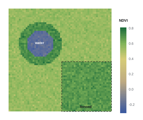
Remote sensing has limits. Clouds and smoke block optical sensors; NDVI saturates in dense vegetation and responds to soil background in sparse vegetation; and images must be corrected for atmospheric effects and sensor differences before comparing dates. Above all, remote sensing products must be validated against field measurements. The team relates NDVI to Robel pole readings and clipped biomass from lesson 8 at sample points, so that a satellite index can be translated into ecologically meaningful units across the whole station.
Species distribution models
Species distribution models relate known occurrences of a species to environmental variables, such as climate, land cover and terrain, and predict where conditions are suitable. Methods range from generalized linear and additive models with presence and absence data, through MaxEnt and other machine-learning methods for presence-only data, to joint models of many species. They are used to map habitat for species at risk, predict invasions and project range shifts under climate change. Their main pitfalls are sampling bias in occurrence records, which concentrate near roads and cities, predicting into conditions unlike those used to fit the model, ignoring dispersal limits and biotic interactions, and spatial autocorrelation that makes models look more accurate than they are unless validated with spatially separate data.
| Tool | What it gives | Typical data | Main caution |
|---|---|---|---|
| Moran's I and correlograms | Degree and scale of autocorrelation | Values at mapped sample points | Depends on the weights chosen |
| Semivariogram and kriging | Range, sill, nugget; interpolated maps | Many georeferenced measurements | Assumes stationarity |
| Landscape metrics | Composition and configuration of habitat | Land cover rasters | Scale-dependent and correlated |
| GIS overlay and buffers | Covariates around each site | Vector and raster layers | Coordinate systems must match |
| NDVI and other indices | Vegetation greenness over space and time | Landsat, Sentinel-2, drones | Clouds, saturation, need validation |
| Species distribution models | Maps of habitat suitability | Occurrences plus environmental layers | Sampling bias, extrapolation |
Worked problem
Choosing sample spacing from a semivariogram
A pilot semivariogram of edge vegetation height has a nugget of 0.15, a sill of 1.0 and a range of 80 m. Sam proposes quadrats every 10 m along 200 m transects. What do these numbers imply?
Show solution
- Quadrats 10 m apart are well within the 80 m range, so neighboring quadrats are strongly correlated and partly redundant.
- The effective number of independent observations per transect is much smaller than 20.
- A nugget of 0.15 of the sill means about 15 percent of the variance is at scales below 10 m or is measurement error.
- Options: space quadrats further apart, put more effort into additional transects or wetlands, or keep the spacing to map fine-scale pattern and analyze with a spatial correlation structure.
Answer: With an 80 m range, 10 m spacing gives highly correlated samples; effort is better spent on more independent transects unless fine-scale mapping is the goal.
Common mistakes
MistakeTreating nearby samples as independent.
InsteadMeasure autocorrelation and use spatial models or spacing beyond the range.
MistakeReporting dozens of landscape metrics.
InsteadChoose a few interpretable, weakly correlated metrics at justified scales.
MistakeCombining GPS points and maps in different datums.
InsteadRecord and match coordinate reference systems.
MistakeTreating NDVI as biomass without field validation.
InsteadCalibrate indices against field measurements.
MistakeValidating species distribution models with random hold-out points.
InsteadUse spatially blocked validation to avoid overoptimism.
Summary and key terms
- Spatial autocorrelation is both information about process scale and a threat to independence.
- Moran's I and correlograms measure autocorrelation; semivariograms describe its nugget, sill and range.
- Landscape composition and configuration are summarized by metrics that depend on grain and extent.
- GIS combines vector and raster layers; coordinate reference systems must be recorded and matched.
- NDVI from Landsat and Sentinel-2 tracks vegetation, but needs field validation.
- Species distribution models map habitat suitability, with pitfalls of bias, extrapolation and autocorrelation.
- spatial autocorrelation
- Similarity of values at nearby locations beyond what is expected by chance.
- Moran's I
- An index of spatial autocorrelation based on weighted cross-products of deviations.
- correlogram
- A plot of autocorrelation against distance class.
- semivariogram
- A function giving half the mean squared difference between values as a function of separation distance.
- range
- The distance beyond which values are no longer autocorrelated.
- nugget
- Semivariance at zero distance, from measurement error and fine-scale variation.
- landscape metric
- A quantitative measure of landscape composition or configuration.
- coordinate reference system
- The datum and projection that give coordinates their meaning.
- NDVI
- The normalized difference vegetation index, (NIR - Red)/(NIR + Red).
- species distribution model
- A model relating species occurrences to environmental variables to predict suitable habitat.
Practice problems
Work each problem on paper first, then reveal the answer to check.
A Moran's I of 0.45 with p = 0.002 means what?
Show answer
Strong positive autocorrelation: similar values cluster in space.
What does a large nugget relative to the sill suggest?
Show answer
Much variation occurs at scales finer than the sampling interval, or there is large measurement error.
A pixel has NIR reflectance 0.40 and red 0.08. What is its NDVI?
Show answer
0.32 / 0.48 = 0.67.
Why might a 90 m grain map show fewer grassland patches than a 30 m map?
Show answer
Small patches merge or disappear when cells are aggregated.
Which satellites provide free 10 m multispectral imagery?
Show answer
Copernicus Sentinel-2.
What is a common error when overlaying GPS points on maps?
Show answer
Mismatched datums or projections.
Why validate NDVI against Robel readings?
Show answer
To translate the index into ecologically meaningful vegetation structure.
Name one pitfall of species distribution models built from community science records.
Show answer
Sampling bias toward roads and cities.
Lesson quiz · 5 questions
Score 60% or more to complete this lesson.
Create a free account to save your progress, take quizzes and earn a certificate.