Sampling designs

You can almost never measure everything. There are too many plants along the station's wetland edges to measure each one, too many square meters of pasture to search for nests, too many wetlands to visit every week. Field ecology therefore relies on sampling: measuring a subset of units chosen so that the subset tells you about the whole. The rules that govern how to choose that subset come from survey sampling theory, developed largely for human populations and agriculture, and they apply with special force in ecology, where organisms are patchy and crews are tempted to sample where it is easy. This lesson covers the main sampling designs, the choice of plot size and shape, transects and plotless methods, and the problem of detectability that sets up the next two lessons.

Populations, frames and units

The target population is the set of things you want to learn about, such as all wetland edges in the station's grazed pastures. The sampling frame is the list or map from which you actually draw your sample, such as a GIS layer of wetland polygons. Sampling units are the things you select and measure: wetlands, quadrats, points, transects or individual plants. Inference from a sample extends only to the frame it was drawn from. If the GIS layer omits wetlands smaller than 0.1 hectare, which in prairie landscapes are the most numerous and the first to be drained or cultivated, conclusions do not cover them. Defining the frame honestly is as important as choosing the design.

Design-based inference treats the population values as fixed and the sample as random: the probability of each unit being selected is known from the design, and that probability is the basis for estimates and their uncertainty. Model-based inference instead treats the values as random outcomes of a statistical model and can use convenient samples if the model is right. Most ecologists mix the two, but design-based thinking guards against the most common failure in field surveys: sampling units that are easy to reach and assuming they represent the rest. Roadside sites, for example, are often wetter, more disturbed and more invaded by weeds than interior sites.

Simple random sampling

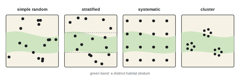
In simple random sampling every possible sample of size \(n\) has the same chance of selection. You might number all 412 wetlands in the frame and select 40 with a random number generator, or place quadrats at random coordinates within a study area. The sample mean is an unbiased estimate of the population mean, and its standard error, with a finite population correction when the sample is a large fraction of the population, is

where \(N\) is the population size and \(s^2\) the sample variance. Simple random sampling is the benchmark, but it can leave large areas unsampled by chance and, when the population contains distinct habitats, it wastes effort on the common habitat and undersamples the rare one.

Stratified sampling

Stratified random sampling divides the population into strata, groups that are internally similar and differ from one another, and samples randomly within each. In the station landscape, wetlands might be stratified by permanence class, since temporary, seasonal and semi-permanent wetlands have very different vegetation and water regimes. The overall mean is a weighted average of stratum means, with weights equal to the stratum's share of the population, and the variance is the weighted sum of within-stratum variances. Because variation among strata is removed, stratification can greatly improve precision when strata differ. It also guarantees that every stratum is sampled, allows separate estimates for each, and lets you sample rare but important strata more intensively.

How many units to put in each stratum? Proportional allocation samples each stratum in proportion to its size. Neyman allocation puts more effort where strata are both large and variable, allocating in proportion to \(N_h s_h\), the stratum size times its standard deviation; if costs differ among strata, allocation in proportion to \(N_h s_h / \sqrt{c_h}\), where \(c_h\) is the cost per unit, is optimal. Pilot data provide the standard deviations.

# Stratified vs simple random sampling of wetland-edge plant cover (synthetic population).
import numpy as np
rng = np.random.default_rng(4)
strata = {'temporary': (220, 18, 12), 'seasonal': (140, 42, 15), 'semi-permanent': (52, 71, 9)}  # N, mean %, SD
pop, lab = [], []
for name, (N, mu, sd) in strata.items():
    vals = np.clip(rng.normal(mu, sd, N), 0, 100)
    pop.append(vals); lab += [name] * N
pop = np.concatenate(pop); lab = np.array(lab); N = len(pop); n = 40
print(f"population: {N} wetlands, true mean cover {pop.mean():.1f}%")
def srs():
    return rng.choice(pop, n, replace=False).mean()
def stratified(alloc):
    est = 0.0
    for name, nh in alloc.items():
        vals = pop[lab == name]
        est += len(vals) / N * rng.choice(vals, nh, replace=False).mean()
    return est
sds = {k: pop[lab == k].std() for k in strata}
Nh = {k: (lab == k).sum() for k in strata}
prop = {k: max(2, round(n * Nh[k] / N)) for k in strata}
w = {k: Nh[k] * sds[k] for k in strata}
neyman = {k: max(2, round(n * w[k] / sum(w.values()))) for k in strata}
print("proportional allocation:", prop, " Neyman allocation:", neyman)
for name, f in [('simple random', srs), ('stratified, proportional', lambda: stratified(prop)), ('stratified, Neyman', lambda: stratified(neyman))]:
    ests = np.array([f() for _ in range(4000)])
    print(f"{name:26s} mean of estimates {ests.mean():5.1f}%, standard error {ests.std():.2f}")

population: 412 wetlands, true mean cover 33.7%
proportional allocation: {'temporary': 21, 'seasonal': 14, 'semi-permanent': 5}  Neyman allocation: {'temporary': 20, 'seasonal': 16, 'semi-permanent': 4}
simple random              mean of estimates  33.8%, standard error 3.19
stratified, proportional   mean of estimates  33.7%, standard error 1.84
stratified, Neyman         mean of estimates  33.7%, standard error 1.84

All three designs are unbiased, but the stratified designs give much smaller standard errors because most of the variation in cover lies between permanence classes. With the same 40 wetlands, the team gets a far more precise estimate simply by using information it already had in the GIS layer.

Systematic, cluster and adaptive designs

Systematic sampling places units at regular intervals from a random start: quadrats every 20 meters along a transect, or points on a 250-meter grid. It is simple to lay out, spreads effort evenly and often gives better precision than simple random sampling because it covers gradients. Its risks are periodicity, if the environment repeats at the same interval as the sampling, such as rows of a planted shelterbelt or ridges and swales, and the lack of an exact variance formula; in practice, treating a systematic sample as random usually gives a conservative variance. Many large monitoring programs use systematic grids with random starts, such as forest inventory plots and the hexagon grids of some national surveys.

Cluster sampling selects groups of units, such as all quadrats in randomly chosen wetlands, because travel between clusters is costly and measuring within a cluster is cheap. Two-stage sampling selects clusters and then subsamples within them, which is what the grazing study does: wetlands are the primary units and quadrats the secondary units. Because units within a cluster tend to be similar, a cluster sample carries less information than the same number of independent units; the design effect quantifies how much.

Adaptive cluster sampling, developed by Steven Thompson in the 1990s, is designed for rare, clumped populations such as a rare plant or invasive species patch. You start with a random sample of units; whenever a unit contains the species, you also sample its neighboring units, and so on until no new occupied units are found. This concentrates effort where the species is, while modified estimators keep the estimate unbiased.

Quadrats: size and shape

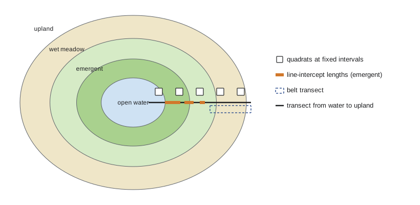
A quadrat is a frame of fixed area, often square, within which you count, measure or estimate the cover of organisms. Choosing its size involves trade-offs. Small quadrats are quick to search thoroughly and allow many replicates, but many will be empty for sparse species and the counts will be highly variable. Large quadrats contain more individuals, but searching them is slow and error-prone, and edge decisions, whether a plant on the boundary is in or out, become a source of bias. A traditional approach plots a statistic such as the number of species against quadrat area and picks the size where the curve starts to level off, but the right size really depends on the organism and question: 0.1 square meters for mosses, 0.25 to 1 square meter for grassland plants, 10 by 10 meters for shrubs and 20 by 20 or larger for trees.

Shape matters too. Long, thin rectangular plots cross more environmental variation and usually capture more heterogeneity than squares of the same area, which reduces variance among plots, but they have more edge relative to area, so boundary errors are more frequent. Circular plots minimize edge and are easy to lay out from a center stake with a measured cord, which is why forest inventories often use them.

Transects

A transect is a line along which sampling is done. Belt transects are long thin plots, such as 2 by 50 meters, in which everything is counted. Line-intercept transects measure the length of the line covered by each species or cover type, a fast and objective way to estimate cover of shrubs, bare ground or emergent vegetation: cover is the total intercepted length divided by the transect length. Point-intercept methods record what touches a pin dropped at fixed intervals along the line. Transects running from the open water of a wetland outward across the edge into upland are ideal for sampling gradients, since the vegetation of pothole wetlands is arranged in concentric zones from submerged plants through emergent cattails and bulrushes to sedges, wet meadow and upland grassland.

# Line-intercept estimate of emergent vegetation cover along wetland-edge transects.
import numpy as np
rng = np.random.default_rng(9)
L = 50.0                                  # transect length, m
covers = []
for t in range(8):                        # 8 transects in one wetland
    x, segs = 0.0, []
    while x < L:
        gap = rng.exponential(3.0); seg = rng.exponential(2.2)
        start = x + gap; end = min(start + seg, L)
        if start < L: segs.append((start, end))
        x = end
    covers.append(sum(e - s for s, e in segs) / L)
covers = np.array(covers)
se = covers.std(ddof=1) / np.sqrt(len(covers))
print("cover per transect:", " ".join(f"{c:.2f}" for c in covers))
print(f"mean emergent cover = {covers.mean():.2f} (SE {se:.3f}); transects, not segments, are the replicates")

cover per transect: 0.48 0.53 0.40 0.33 0.40 0.51 0.25 0.52
mean emergent cover = 0.43 (SE 0.035); transects, not segments, are the replicates

Plotless methods

In forests and shrublands, laying out large plots is slow, so ecologists developed distance methods that estimate density from distances between points and plants. The best known is the point-centered quarter method of Cottam and Curtis, from the 1950s. At each sampling point, the area around it is divided into four quarters, and the distance to the nearest plant in each quarter is measured. If plants are randomly distributed, density is estimated as one over the square of the mean distance: \(\hat{D} = 1/\bar{r}^2\). The method is fast and needs no plot boundaries, but it is biased when plants are clumped or regular, which is common, and modern variants correct for this. Basal area by prism, covered in lesson 8, is another plotless technique.

# PCQ (point quarter) estimate of aspen stem density in a grove (synthetic, random stems).
import numpy as np
rng = np.random.default_rng(21)
true_density = 0.12                                   # stems per m2 (1,200 per hectare)
side = 200.0
stems = rng.uniform(0, side, (rng.poisson(true_density * side**2), 2))
dists = []
for _ in range(25):                                   # 25 sampling points away from edges
    p = rng.uniform(40, side - 40, 2)
    d = stems - p
    for qx, qy in [(1, 1), (-1, 1), (-1, -1), (1, -1)]:
        mask = (np.sign(d[:, 0]) == qx) & (np.sign(d[:, 1]) == qy)
        dists.append(np.hypot(*d[mask].T).min())
rbar = np.mean(dists)
print(f"mean point-to-stem distance = {rbar:.2f} m from {len(dists)} quarters")
print(f"estimated density = {1 / rbar**2:.3f} stems/m2 = {10000 / rbar**2:,.0f} per hectare (true 1,200)")

mean point-to-stem distance = 2.66 m from 100 quarters
estimated density = 0.141 stems/m2 = 1,412 per hectare (true 1,200)

Detectability

Every method so far assumes that if an organism is in a sampling unit, you will find it. For plants in a small quadrat that is nearly true, although even botanists miss small or cryptic species. For animals it is rarely true. A sparrow singing 30 meters away may be heard every time; one 150 meters away may be missed half the time; a silent female on a nest will almost always be missed. A count is therefore the product of how many animals are present and the probability of detecting each one: \(E(C) = N p\). If detection probability differs among habitats, observers, weather or seasons, raw counts compare detectability as much as abundance. In the grazing study, taller vegetation after fencing could make sparrows harder to see, so a raw count could fall even if the number of birds rose.

There are two broad responses. One is to standardize methods so that detection is as constant as possible: same observers, same time of morning, same weather limits, same duration. The other is to estimate detection probability directly and correct for it. Lessons 5 and 6 cover the main estimation methods: distance sampling, which models how detection falls with distance; mark–recapture, which uses repeated captures of known individuals; removal sampling; and occupancy and repeated-count models, which use repeated visits to the same sites. A good field design anticipates detectability from the start, because the extra data these methods need, such as distances, repeated visits or marked individuals, must be collected in the field.