
BIOL-430 · Lesson 1 of 12 · 28 min
Asking ecological questions in the field
Field ecology is the craft of answering questions about living things where they actually live. A laboratory lets you hold temperature constant, choose your organisms and repeat an experiment on demand. A wetland, a forest edge or a pasture gives you none of those luxuries: the weather changes, animals move, plants grow on their own schedule, and the thing you are measuring may be hiding from you. What the field offers instead is realism. The answers you get describe nature as it is, with all its interacting causes, at the scales where conservation, agriculture and land management actually happen. This course is about doing that work well, from the first question to a published, reusable data set.
The course builds on BIOL-208, which introduced populations, communities and ecosystems, and on STAT-151, which introduced study design, regression and hypothesis tests. BIOL-367 used several field tools in a conservation setting, including diversity indices, rarefaction, Chao1 and simple occupancy estimates; we refer back to those rather than repeating them. Here the emphasis is on how field data are collected and analyzed, and on the judgment that turns a pile of numbers into defensible conclusions.
A running example
Throughout the course we follow one invented research program at the invented Otter Tail Prairie Field Station, in the prairie pothole country near Fergus Falls, Minnesota. The landscape is a mosaic of tallgrass prairie remnants, pasture, cropland, oak and aspen groves, and thousands of small prairie pothole wetlands, the shallow depressions left by the last glaciation that fill with snowmelt each spring. A cooperating ranch is changing how it grazes cattle: starting in the third year of the study, it will fence the margins of some wetlands and move cattle through paddocks on a rotation instead of grazing them season-long. The research team, led by an invented ecologist, Dr. Amara Okafor, wants to know what that change does to wetland-edge vegetation, grassland birds, small mammals and amphibians.
The team includes two graduate students, Liam Tremblay and Priya Nair, and a field technician, Sam Whitford. All of the data in this course are synthetic, generated by seeded code so that every number can be reproduced, but the methods, problems and decisions are the ones real field crews face. Each lesson adds a piece: designing the grazing study, getting permits and keeping the crew safe, sampling vegetation, counting birds and mice, measuring diversity, tracking deer, mapping the landscape from satellites, analyzing the results and, in the capstone, writing a proposal for long-term monitoring.
From pattern to question
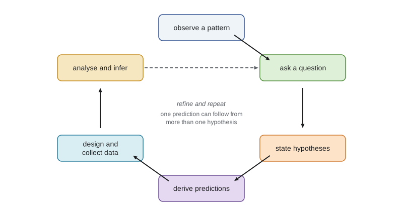
Most field studies begin with a pattern someone noticed. A rancher mentions that ducks seem scarcer around heavily grazed sloughs. A naturalist sees more bobolinks in fields hayed late. A graduate student notices that sedges grow taller inside a fence that was put up to keep cattle off a dugout. Patterns are where curiosity starts, but a pattern is not yet a question you can answer. Turning it into one means deciding exactly what you want to know, about which organisms, at what place and scale, and what kind of answer would satisfy you.
Ecologists find it useful to separate three kinds of questions. Descriptive questions ask what is there and how much: how many breeding pairs of savannah sparrows use the station's pastures, or what fraction of wetlands hold calling chorus frogs. Comparative or correlational questions ask how things vary together: are wetlands with more emergent vegetation used by more frogs? Causal questions ask what happens if something changes: does fencing wetland margins increase plant height and cover at the edge? Each kind is legitimate, and good description is badly underrated, but each needs different evidence. A causal claim needs either an experiment or a careful argument that alternative explanations have been ruled out.
A good field question is specific, answerable with the time and money available, and interesting to someone beyond the person asking it. Compare 'How does grazing affect wetlands?' with 'Does excluding cattle from a 10-meter band around prairie pothole wetlands increase the mean height of emergent vegetation at the wetland edge within two growing seasons?' The second question names the treatment, the response, the location, the scale and the time frame. It also tells you what to measure, where and when, which is the point.
Hypotheses and predictions
A hypothesis is a proposed explanation; a prediction is what you should observe if the hypothesis is true. The distinction matters because the same prediction can follow from several hypotheses. Suppose vegetation is taller inside fenced wetland margins. The obvious hypothesis is that cattle grazing and trampling reduce plant height, so removing cattle lets plants grow. But perhaps the ranch chose to fence the wettest margins, where plants grow tall anyway, or perhaps fences change snow drifting and so soil moisture. Each hypothesis predicts taller plants inside fences; they differ in other predictions. The grazing hypothesis predicts that the difference should appear only after fencing, and that grazed plants should show bite marks; the site-selection hypothesis predicts the difference existed before fencing. Designing a study means finding predictions that distinguish between competing explanations.
The classical framework for this is Platt's strong inference and Chamberlin's method of multiple working hypotheses: list every plausible explanation, derive predictions that separate them and collect data that can eliminate some. In practice, ecological processes are rarely all-or-nothing. Grazing probably does reduce plant height, and fences probably were put in particular places, and both matter. Modern field ecology therefore tends to ask how large each effect is, with what uncertainty, rather than whether an effect exists at all. That shift, from asking whether to asking how much, runs through this course.
Kinds of field studies
Field studies fall along a range of control. At one end are purely observational studies, in which the researcher measures what is there without changing anything: surveys of bird abundance across pastures, or measurements of wetland water chemistry. At the other are manipulative experiments, in which the researcher assigns treatments at random to units: fencing randomly chosen wetland margins, adding nutrients to plots or removing a predator from enclosures. Between them are natural experiments, where something outside the researcher's control changes some units and not others, such as a wildfire, a flood, a road built through part of a study area or a policy that applies on one side of a border. Each step toward control buys stronger causal inference at the cost of realism, scale or feasibility.
| Type | Example from the running study | Strengths | Weaknesses |
|---|---|---|---|
| Descriptive survey | Counting breeding birds on 60 points across the station | Large areas, real conditions, baseline for later change | Cannot say why patterns occur |
| Correlational (observational) study | Relating frog occupancy to emergent vegetation across 40 wetlands | Reveals associations across natural gradients | Confounding: other variables vary along with the one of interest |
| Natural experiment | Comparing wetlands burned by a 2024 grass fire with unburned ones | Realistic, large-scale disturbance; can be the only option | No randomization; burned and unburned sites may differ |
| Manipulative experiment | Randomly assigning fencing to wetland margins | Strongest causal inference within its scale | Often small, short or expensive; treatments may be unrealistic |
| Before–after–control–impact (BACI) study | Measuring fenced and unfenced wetlands before and after the ranch changes | Handles pre-existing differences and year effects | Needs data before the change; treatment often not randomized |
Experiments in ecology come in different sizes. Microcosm experiments in jars or tanks give precise control but small scale. Field plot experiments, such as clipping or fertilizing one-square-meter plots, are realistic but limited in extent. Whole-ecosystem experiments, such as the lake manipulations at the IISD Experimental Lakes Area in northwestern Ontario, which showed in the 1970s that phosphorus drives algal blooms, can change management decisions because their scale matches the scale of the problem. When an experiment is impossible because the treatment is too large, too slow or unethical, ecologists combine observational studies, natural experiments and models, an approach sometimes called weight of evidence.
Confounding and causal inference
The central challenge of observational field data is confounding: a third variable affects both the factor you care about and the response. Ranchers do not place cattle at random. Heavily grazed pastures may be closer to water, on richer soils or lower in the landscape. If wetter sites have both more cattle and taller vegetation, a naive comparison could show that grazing goes with taller plants, the opposite of the true effect. Randomization solves this problem in experiments because, on average, it balances every confounder, measured or not, across treatments. In observational studies you can only adjust for confounders you have measured, using regression, matching or stratification, and you must argue that unmeasured confounders are unlikely to explain the result.
Causal diagrams, sometimes called directed acyclic graphs, help here. Draw an arrow from each variable to the variables it affects: soil moisture to grazing intensity (cattle concentrate near water) and soil moisture to plant height; grazing to plant height. The diagram shows that to estimate the effect of grazing on height, you must account for soil moisture, a so-called back-door path. It also warns against adjusting for variables that lie on the causal path, such as bare ground created by trampling, which would hide part of the effect you want to measure.
# Confounding: grazing intensity and plant height both depend on soil moisture.
import numpy as np
rng = np.random.default_rng(430)
n = 120                                     # wetland edges surveyed
moisture = rng.uniform(10, 50, n)           # volumetric soil moisture, %
grazing = 0.6 * moisture + rng.normal(0, 6, n)   # cattle concentrate near water (AUM index)
height = 20 + 1.5 * moisture - 0.8 * grazing + rng.normal(0, 6, n)  # true grazing effect -0.8 cm per unit
X1 = np.column_stack([np.ones(n), grazing])
b1 = np.linalg.lstsq(X1, height, rcond=None)[0]
X2 = np.column_stack([np.ones(n), grazing, moisture])
b2 = np.linalg.lstsq(X2, height, rcond=None)[0]
print(f"correlation of grazing with moisture: {np.corrcoef(grazing, moisture)[0, 1]:.2f}")
print(f"naive slope of height on grazing:      {b1[1]:+.2f} cm per unit")
print(f"slope adjusted for soil moisture: {b2[1]:+.2f} cm per unit (true value -0.80)")correlation of grazing with moisture: 0.79 naive slope of height on grazing: +0.62 cm per unit slope adjusted for soil moisture: -0.76 cm per unit (true value -0.80)
The simulation shows how badly confounding can mislead. Because cattle concentrate where soil is wet and wet soil grows tall plants, the naive regression suggests that grazing increases height. Adjusting for moisture recovers an estimate close to the true negative effect. In real data you never know the true value, and you can never be sure you measured every confounder, which is why the design of a study matters more than any later analysis.
Scale
Every ecological pattern depends on the scale at which you look. Scale has two components: grain, the size of the smallest unit you measure, such as a 0.5 by 0.5 meter quadrat or a 10-meter satellite pixel; and extent, the total area or time span covered, such as one pasture or the whole prairie pothole region, one summer or forty years. Processes operate at characteristic scales: trampling acts at the scale of hoofprints, cattle distribution at the scale of paddocks and water sources, and climate at the scale of regions. A study whose grain is too coarse will miss fine-scale processes; one whose extent is too small will miss broad-scale ones and may not generalize. Lesson 10 returns to scale with spatial statistics.
Time matters too. A single field season may happen to be a drought year, as several recent prairie summers have been, and wetland plants and amphibians respond very differently in wet and dry years. Effects of grazing changes on vegetation may appear within one or two seasons, but effects on soil carbon, shrub encroachment or bird populations may take a decade. Short studies are not worthless, but conclusions should be limited to the conditions and time span actually observed.
Precision and sample size
Field data are noisy, and the most common reason a field study fails to answer its question is too few replicates. The uncertainty of an estimated mean shrinks with the square root of the sample size: the standard error is \(SE = s/\sqrt{n}\), where \(s\) is the standard deviation among units. Halving the width of a confidence interval requires four times as many units. Because travel, permits and labor are the main costs of fieldwork, decisions about how many sites to visit, and how much effort to spend at each, are often the most important design decisions you will make.
# How the precision of a mean vegetation height depends on the number of quadrats.
import numpy as np
rng = np.random.default_rng(31)
population = rng.gamma(shape=4, scale=12, size=5000)   # heights (cm) along all wetland edges
print(f"true mean height: {population.mean():.1f} cm, SD {population.std():.1f} cm")
for n in (5, 10, 20, 40, 80, 160):
    widths = []
    for _ in range(2000):
        s = rng.choice(population, n, replace=False)
        widths.append(2 * 1.96 * s.std(ddof=1) / np.sqrt(n))
print(f"n = {n:3d} quadrats: average 95% CI width = {np.mean(widths):5.1f} cm")true mean height: 48.4 cm, SD 24.6 cm n = 5 quadrats: average 95% CI width = 39.7 cm n = 10 quadrats: average 95% CI width = 29.1 cm n = 20 quadrats: average 95% CI width = 21.2 cm n = 40 quadrats: average 95% CI width = 15.0 cm n = 80 quadrats: average 95% CI width = 10.7 cm n = 160 quadrats: average 95% CI width = 7.6 cm
The output shows the diminishing returns: going from 5 to 20 quadrats narrows the interval a lot; going from 80 to 160 helps much less. A pilot season is the best way to estimate the variability, \(s\), that drives these calculations. Lesson 2 extends this idea to power analysis, asking how many units are needed to detect an effect of a given size.
Effect sizes and what counts as important
Statistical significance tells you whether an effect is distinguishable from zero given your data; it does not tell you whether the effect matters. With enough replicates, a 2 percent change in plant height can be highly significant and ecologically trivial; with too few, a 40 percent change can be non-significant and very important. Field ecologists therefore report effect sizes, such as the difference in means, a ratio, a slope or a standardized difference, with confidence intervals, and they decide before collecting data what size of effect would matter for the question. For the grazing study, the team might decide that a 10-centimeter increase in edge vegetation height, which is about the difference that affects nest concealment for ground-nesting ducks and songbirds, is the smallest effect worth detecting.
Pre-registration, writing down your hypotheses, design and analysis plan before you see the data and archiving it with a time stamp, is becoming more common in ecology. It guards against the temptation to try many analyses and report the one that gives the most exciting result. It does not forbid exploration; it separates confirmatory tests, planned in advance, from exploratory findings, which are honest but need confirmation. Lesson 12 discusses how to write a pre-registered field study proposal.
Worked problem
Sharpening a question
Liam proposes to study whether grazing affects grassland birds at the station. Turn this into a specific, answerable question, list at least two competing hypotheses for a possible pattern and state one prediction that would distinguish them.
Show solution
- Specify organism, response, treatment, place and time: does the density of breeding savannah sparrows on territories within 200 meters of pothole wetlands differ between season-long and rotationally grazed pastures at the station over two breeding seasons?
- Hypothesis 1: rotational grazing leaves taller, denser residual cover, which sparrows prefer for nesting, so density is higher in rotational pastures.
- Hypothesis 2: the ranch converted its most productive pastures to rotational grazing first, and those pastures already had more sparrows.
- Distinguishing prediction: if hypothesis 1 holds, sparrow density should increase in converted pastures after the change relative to unconverted ones; if hypothesis 2 holds, density should already be higher in those pastures before conversion and not change differentially.
- This points directly to a before–after–control–impact design, the subject of lesson 2.
Answer: A specific question names the species, response, treatment, place and period; competing hypotheses are separated by asking whether the difference appears only after the management change.
Common mistakes
MistakeStarting fieldwork with a vague question and hoping a pattern will emerge.
InsteadDefine the response, treatment, scale and time frame first, so the data you collect can answer something.
MistakeTreating a correlation from an observational survey as proof of cause.
InsteadConsider confounders, use causal diagrams and look for designs or data that rule out alternatives.
MistakeAssuming a significant p-value means an important effect.
InsteadReport effect sizes with confidence intervals and decide in advance what size of effect matters.
MistakeGeneralizing one season or one site to the whole region.
InsteadLimit conclusions to the scale and conditions sampled, and replicate across years and places when possible.
MistakeAdjusting for every available variable in an observational analysis.
InsteadAdjust for confounders, but not for variables on the causal path, which hide part of the effect.
Summary and key terms
- Field ecology trades the control of the laboratory for realism at the scales where management happens.
- Good questions are specific about organism, response, treatment, place, scale and time.
- Hypotheses explain; predictions follow from them, and strong designs test predictions that separate competing hypotheses.
- Studies range from descriptive surveys through natural experiments to randomized manipulative experiments, trading realism for causal strength.
- Confounding is the main threat in observational data; randomization handles it in experiments.
- Precision grows with the square root of sample size, and effect sizes matter more than p-values.
- hypothesis
- A proposed explanation for an observed pattern.
- prediction
- An observable outcome expected if a hypothesis is true.
- observational study
- A study in which the researcher measures existing variation without assigning treatments.
- manipulative experiment
- A study in which treatments are assigned by the researcher, ideally at random.
- natural experiment
- A comparison exploiting a change imposed by events outside the researcher's control.
- confounding
- Distortion of an estimated effect by a variable that influences both the factor of interest and the response.
- grain
- The size of the smallest sampling unit or resolution of measurement.
- extent
- The total area or time span covered by a study.
- effect size
- The magnitude of a difference or relationship, independent of sample size.
- pre-registration
- Recording hypotheses, design and analysis plans before data are collected or examined.
Practice problems
Work each problem on paper first, then reveal the answer to check.
Classify this question: what fraction of the station's wetlands support breeding wood frogs?
Show answer
Descriptive.
Why does randomization protect against confounding?
Show answer
On average it balances all variables, measured and unmeasured, across treatments.
If the standard deviation of plant height is 20 cm, what is the standard error of a mean from 25 quadrats?
Show answer
20 / 5 = 4 cm.
How many quadrats would you need to halve that standard error?
Show answer
Four times as many: 100.
Give an example of a natural experiment in prairie ecology.
Show answer
Comparing wetlands burned by a wildfire with similar unburned wetlands, or before and after a drought.
In the grazing study, why should you not adjust for bare ground when estimating the effect of grazing on plant height?
Show answer
Bare ground is caused by trampling and lies on the causal path, so adjusting for it removes part of the grazing effect.
What is the difference between grain and extent?
Show answer
Grain is the resolution of measurement; extent is the total area or time covered.
What does pre-registration guard against?
Show answer
Selectively reporting whichever of many analyses gives the most striking result.
Lesson quiz · 5 questions
Score 60% or more to complete this lesson.
Create a free account to save your progress, take quizzes and earn a certificate.