
BIOL-430 · Lesson 8 of 12 · 25 min
Vegetation, habitat and environmental measurements
Animals respond to habitat, and habitat is mostly vegetation and the physical environment that shapes it. The grazing study's central prediction is about vegetation: that fencing wetland margins will make edge plants taller and denser. Measuring that well requires standard methods for cover, height and structure, for trees and shrubs where groves meet the wetlands, and for the soils, water and microclimate that drive plant growth. This lesson covers the field techniques ecologists use for those measurements, how to make them repeatable across observers and years, and how loggers and phenology networks extend measurements through time.
Cover estimation
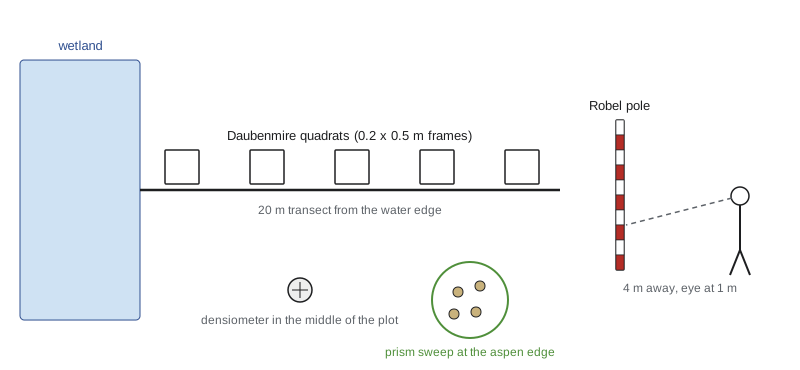
Cover is the proportion of ground covered by the vertical projection of a plant's canopy, and it is the most common measure of plant abundance in grasslands and wetlands, where counting individuals of clonal grasses and sedges is impractical. Visual estimates in quadrats are fast but vary among observers, especially for intermediate values. Cover-class systems reduce that variation by asking observers to choose a class rather than a precise percentage. The Daubenmire system, published in 1959 and widely used in western North American rangelands, uses six classes: 0 to 5, 5 to 25, 25 to 50, 50 to 75, 75 to 95 and 95 to 100 percent, analyzed using class midpoints. The Braun-Blanquet scale, common in European phytosociology, combines cover with abundance. Because total cover of all species can exceed 100 percent where canopies overlap, cover of each species is estimated separately.
Point-intercept methods are more objective. A pin or laser is lowered at regular points, along a transect or through a frame, and every species touching it is recorded; cover is the fraction of points with a hit. With enough points, often 100 or more per plot, point-intercept data have less observer bias than visual estimates and can distinguish layers. They are slower and miss rare species, so many protocols combine point-intercept cover with a search of the plot for additional species.
# Daubenmire cover classes to mean cover, and observer agreement on the same quadrats (synthetic).
import numpy as np
rng = np.random.default_rng(81)
bins = [0, 5, 25, 50, 75, 95, 100]; mids = [2.5, 15, 37.5, 62.5, 85, 97.5]
true = np.clip(rng.beta(2, 2.5, 40) * 100, 0, 100)              # true sedge cover in 40 quadrats
def visual(err):
    return np.clip(true + rng.normal(0, err, true.size), 0, 100)
for name, err in [('Liam', 8), ('Priya', 14)]:
    est = visual(err)
    cls = np.digitize(est, bins[1:-1])
    mid = np.array(mids)[cls]
    print(f"{name:5s}: visual mean {est.mean():5.1f}%, class-midpoint mean {mid.mean():5.1f}%  (true {true.mean():.1f}%)")
a = np.digitize(visual(8), bins[1:-1]); b = np.digitize(visual(14), bins[1:-1])
print(f"same Daubenmire class chosen by both observers in {np.mean(a == b):.0%} of quadrats")
pts = rng.uniform(size=(40, 100)) < true[:, None] / 100           # 100 point-intercepts per quadrat
print(f"point-intercept mean cover {pts.mean() * 100:.1f}%")Liam : visual mean 41.1%, class-midpoint mean 41.6% (true 39.9%) Priya: visual mean 40.2%, class-midpoint mean 39.4% (true 39.9%) same Daubenmire class chosen by both observers in 52% of quadrats point-intercept mean cover 40.6%
Observer differences are a major source of error in vegetation monitoring. Calibration sessions at the start of each season, in which all observers estimate the same quadrats and compare, reduce them; assigning observers so that each one visits plots in every treatment prevents observer effects from being confounded with treatments; and recording observer identity lets analyses account for any remaining differences.
Height, structure and visual obstruction
Height can be measured as the maximum height of each species, the height of the tallest live vegetation touching a measuring stick at fixed points, or a mean of several readings per plot. For wildlife habitat in grasslands, structure matters more than height alone. The Robel pole, introduced by Robel and colleagues in 1970 for prairie grouse habitat, is a pole marked in bands; an observer standing 4 meters away, with eye height 1 meter, records the lowest band not completely hidden by vegetation, from four directions. The reading, called visual obstruction, integrates height and density into one number and correlates closely with the mass of standing vegetation. It is widely used to assess nesting cover for ducks and grassland birds, which makes it the natural response variable for the grazing study.
Residual cover, the standing vegetation left over winter, determines nest concealment in spring, because most prairie ducks and many grassland birds nest before new growth is tall. That is why grazing management in waterfowl habitat often aims to leave a minimum residual height, and why the team measures visual obstruction both in late summer and the following spring.
# Robel pole visual obstruction before and after fencing at 12 impact and 12 control wetlands (synthetic).
import numpy as np
rng = np.random.default_rng(1970)
wet = rng.normal(0, 3, 24)                           # persistent wetland differences (dm)
impact = np.arange(24) < 12
before = 9 + wet + rng.normal(0, 1.5, 24)
after = 9 + wet + rng.normal(0.5, 1.5, 24) + np.where(impact, 4.0, 0.0)
def readings(level):                                  # four directions, read to the nearest 0.5 dm band
    return np.round((level[:, None] + rng.normal(0, 1.2, (24, 4))) * 2) / 2
b, a = readings(before).mean(1), readings(after).mean(1)
d = (a - b)
print(f"mean visual obstruction (dm): impact {b[impact].mean():.1f} -> {a[impact].mean():.1f}, control {b[~impact].mean():.1f} -> {a[~impact].mean():.1f}")
print(f"BACI estimate = {d[impact].mean() - d[~impact].mean():.1f} dm (true 4.0)")mean visual obstruction (dm): impact 7.9 -> 12.3, control 11.4 -> 11.7 BACI estimate = 4.1 dm (true 4.0)
In this synthetic data set the impact wetlands happened to start with less cover than the controls, 7.9 against 11.4 decimeters, which is exactly the situation the BACI design handles: the estimate uses each wetland's change, so the starting difference cancels and the estimate lands close to the true 4-decimeter effect.
Trees and shrubs
Where aspen groves and willow rings border the wetlands, woody vegetation is measured differently. Diameter at breast height (DBH), the stem diameter at 1.3 meters above the ground in Canada and most of the world and at 4.5 feet (1.37 meters) in United States forestry, is measured with a diameter tape that converts circumference to diameter. Basal area, the cross-sectional area of stems at breast height per hectare, is a standard measure of stand density and dominance: each stem contributes \(\pi (\mathrm{DBH}/2)^2\). In plots it is summed over stems and scaled to a hectare.
A faster plotless method uses a wedge prism or angle gauge. The observer stands at a point and looks at each tree through the prism, which offsets the image; trees whose offset image still overlaps the real trunk are counted ('in'), and borderline trees are checked. Each counted tree represents the same basal area per hectare, the basal area factor (BAF) of the prism, so basal area per hectare equals the count times BAF. A BAF 2 metric prism, for example, means each 'in' tree represents 2 square meters per hectare. Prism sweeps are a staple of forest inventory because they take a minute or two per point and automatically sample larger trees more often, in proportion to their importance for basal area.
Canopy cover over wetland margins is measured with a spherical densiometer, a convex or concave mirror with a grid; the observer counts grid points reflecting sky, usually in four directions. Hemispherical photographs taken upward with a fisheye lens and analyzed by software give canopy openness and estimates of light transmission. Shrub density can be measured by counting stems in belt transects, and browse surveys record the proportion of twigs browsed by deer or moose, a useful index of browsing pressure.
# Basal area from a fixed-radius plot and from a prism sweep in an aspen grove (synthetic).
import numpy as np
rng = np.random.default_rng(13)
dbh = rng.gamma(6, 3.0, 45)                       # cm, 45 stems in a 0.04 ha (11.28 m radius) plot
ba_plot = np.sum(np.pi * (dbh / 200) ** 2) / 0.04   # m2 per hectare
print(f"plot: {len(dbh)} stems, mean DBH {dbh.mean():.1f} cm, basal area {ba_plot:.1f} m2/ha, density {len(dbh) / 0.04:,.0f} stems/ha")
BAF = 2.0                                         # metric prism, m2/ha per counted tree
counts = rng.poisson(ba_plot / BAF, 8)             # 8 prism points in the grove
print(f"prism counts at 8 points: {counts.tolist()} -> basal area {counts.mean() * BAF:.1f} m2/ha (SE {counts.std(ddof=1) / np.sqrt(8) * BAF:.1f})")plot: 45 stems, mean DBH 18.1 cm, basal area 33.6 m2/ha, density 1,125 stems/ha prism counts at 8 points: [14, 17, 16, 20, 15, 17, 19, 14] -> basal area 33.0 m2/ha (SE 1.6)
Soils
Soils mediate how grazing and water affect plants. Key field measurements include texture, the proportions of sand, silt and clay, estimated in the field by feel or measured in the laboratory; organic matter and color, recorded against standard color charts; bulk density, the dry mass of soil per volume, which rises when cattle compact soil; and soil moisture, measured gravimetrically by weighing samples before and after drying or with time-domain reflectometry probes that read volumetric water content instantly. Soil pH and salinity matter in prairie wetlands, where evaporation concentrates salts and saline margins support specialized plants such as foxtail barley and Nuttall's alkaligrass.
United States soils are described using USDA Soil Taxonomy, and the Web Soil Survey from the Natural Resources Conservation Service provides county soil maps; the prairie soils of the Minnesota study area are mostly Mollisols, dark, organic-rich soils formed under grassland, with poorly drained hydric soils in and around wetlands, which are a key criterion in federal wetland delineation.
Water and microclimate
Prairie pothole wetlands are defined by their water. Water depth at a fixed staff gauge, recorded on each visit or continuously by a pressure transducer, shows how long each wetland holds water, its hydroperiod, which shapes which plants and amphibians it supports. Water chemistry measurements include temperature, dissolved oxygen, pH, specific conductance (a proxy for salinity), turbidity and nutrients such as nitrogen and phosphorus, which run off from cropland and are concentrated by cattle. Multi-parameter probes measure several of these in seconds but need regular calibration against standard solutions.
Data loggers record temperature, humidity, light or water level every few minutes for months. Small, cheap temperature loggers placed at the ground surface under vegetation reveal microclimates that differ sharply from weather-station records: a tall sedge canopy may be several degrees cooler at midday than grazed turf. Logger data support calculations such as growing degree days, the accumulated warmth above a base temperature that predicts plant and insect development.
# Growing degree days (base 5 C) from ground-surface loggers in fenced and grazed edges (synthetic, May-August).
import numpy as np
rng = np.random.default_rng(5)
days = np.arange(123)                                   # 1 May to 31 August
seasonal = 6 + 12 * np.sin(np.pi * days / 122)
for name, offset_max, offset_min in [('fenced edge (tall sedge)', -2.0, 0.8), ('grazed edge (short turf)', 2.5, -0.6)]:
    tmax = seasonal + 8 + offset_max + rng.normal(0, 3, days.size)
    tmin = seasonal - 6 + offset_min + rng.normal(0, 2.5, days.size)
    gdd = np.cumsum(np.maximum(0, (tmax + tmin) / 2 - 5))
print(f"{name:26s} GDD by 30 June {gdd[60]:5.0f}, by 31 August {gdd[-1]:5.0f}; days above 30 C: {(tmax > 30).sum()}")fenced edge (tall sedge) GDD by 30 June 535, by 31 August 1089; days above 30 C: 1 grazed edge (short turf) GDD by 30 June 653, by 31 August 1301; days above 30 C: 11
Phenology
Phenology, the timing of biological events such as leaf-out, flowering, insect emergence and bird arrival, is among the clearest signals of climate change and is easy to record in the field. Standardized protocols define phenophases, such as first open flower, so that observations are comparable. Long-term records, from Aldo Leopold's Wisconsin farm notes of the 1930s and 1940s to modern networks, show many spring events advancing.
In the United States, the USA National Phenology Network collects standardized observations through its Nature's Notebook program, from volunteers and professionals, on thousands of species, and publishes maps of spring onset; Minnesota observers have contributed long phenology records, including lake ice-out dates kept for more than a century.
| Measurement | Typical method | Unit | Main source of error |
|---|---|---|---|
| Species cover | Daubenmire classes or point intercept | percent | Observer differences |
| Visual obstruction | Robel pole from four directions at 4 m | decimeters | Observer position and eye height |
| Basal area | Fixed plot or wedge prism | m2 per hectare | Borderline trees, slope |
| Canopy cover | Spherical densiometer or hemispherical photo | percent | Sky conditions, operator |
| Soil moisture | Gravimetric or TDR probe | percent by volume or mass | Spatial variation, calibration |
| Water depth and hydroperiod | Staff gauge or pressure logger | cm, days | Gauge movement, logger drift |
| Microclimate | Shielded temperature loggers | degrees C | Radiation shielding, placement |
| Phenology | Standardized phenophase protocols | day of year | Visit frequency |
Worked problem
Converting prism counts and Robel readings
At one grove edge Sam counts 7 trees in a BAF 2 prism sweep. At the wetland edge nearby, the Robel readings from four directions are 3.5, 4.0, 2.5 and 3.0 dm. Report basal area and visual obstruction.
Show solution
- Basal area = count x BAF = 7 x 2 = 14 square meters per hectare.
- Visual obstruction = mean of the four readings = (3.5 + 4.0 + 2.5 + 3.0) / 4 = 3.25 dm.
- Record observer, date and the eye height and distance used, since changing them changes readings.
Answer: 14 m2 per hectare of basal area and a visual obstruction of 3.25 dm.
Common mistakes
MistakeLetting one observer survey all treated plots and another all controls.
InsteadRotate observers across treatments and calibrate them each season.
MistakeRecording total cover only.
InsteadEstimate cover by species and record bare ground and litter separately.
MistakeUsing a different distance or eye height for Robel readings.
InsteadFollow the standard 4 m and 1 m geometry every time.
MistakeRelying on weather-station temperatures for microclimate.
InsteadPlace shielded loggers where organisms live.
MistakeSkipping probe calibration in water chemistry.
InsteadCalibrate multi-parameter probes against standards before each field day.
Summary and key terms
- Cover is estimated visually in classes or objectively by point intercept; observers must be calibrated and balanced across treatments.
- Robel pole visual obstruction integrates height and density and is standard for grassland nesting cover.
- Woody vegetation is measured by DBH, basal area from plots or prisms, canopy cover and browse surveys.
- Soils, water chemistry and hydroperiod drive wetland-edge vegetation and must be measured alongside it.
- Data loggers reveal microclimates and support measures such as growing degree days.
- Phenology networks provide long, standardized records of seasonal timing.
- cover
- The proportion of ground covered by the vertical projection of plant canopies.
- Daubenmire cover classes
- Six cover classes used for visual estimates, analyzed by class midpoints.
- point-intercept method
- Recording plants touching a pin or laser at regular points to estimate cover.
- visual obstruction
- The height of vegetation that hides a marked pole viewed from a standard distance.
- residual cover
- Standing vegetation left from the previous growing season.
- diameter at breast height
- Stem diameter measured at 1.3 m above ground (4.5 ft in US forestry).
- basal area
- Cross-sectional stem area at breast height per unit ground area.
- basal area factor
- The basal area per hectare represented by each tree counted in a prism sweep.
- hydroperiod
- The length of time a wetland holds surface water.
- growing degree days
- Accumulated daily mean temperature above a base, a predictor of development.
Practice problems
Work each problem on paper first, then reveal the answer to check.
A Daubenmire class of 25 to 50 percent is analyzed as what value?
Show answer
The midpoint, 37.5 percent.
A pin frame records sedge at 34 of 100 points. What is sedge cover?
Show answer
34 percent.
Calculate the basal area of one tree with DBH 30 cm.
Show answer
pi x 0.15^2 = 0.071 m2.
A BAF 4 prism counts 5 trees. What is basal area per hectare?
Show answer
20 m2 per hectare.
Why measure residual cover in spring?
Show answer
Early nesting birds rely on last year's vegetation for concealment.
A day has Tmax 22 C and Tmin 8 C. How many growing degree days does it add at base 5 C?
Show answer
(22 + 8)/2 - 5 = 10.
What does specific conductance indicate in a pothole wetland?
Show answer
Salinity, the concentration of dissolved ions.
Why should observer identity be recorded?
Show answer
So observer differences can be checked and accounted for in analysis.
Lesson quiz · 5 questions
Score 60% or more to complete this lesson.
Create a free account to save your progress, take quizzes and earn a certificate.