
BIOL-420 · Lesson 4 of 12 · 26 min
Synaptic transmission
Chemical synapses are where most of the computation in a nervous system happens. They convert an electrical signal into a chemical one and back, they can amplify or attenuate, they change their strength with use, and they are the targets of most drugs that act on the brain. BIOL-350 introduced the sequence of events: an action potential invades the terminal, calcium enters, vesicles fuse and release transmitter, and receptors open on the postsynaptic side. This lesson examines each step quantitatively and molecularly: the quantal nature of release and how it is analyzed, the steep calcium dependence of release, the protein machinery of fusion, the vesicle cycle, short-term plasticity, and the two broad classes of receptors.
Quanta: the unit of release
In the early 1950s Paul Fatt and Bernard Katz, recording from frog neuromuscular junctions, noticed small spontaneous depolarizations of about 0.5 millivolts occurring at random even without nerve stimulation. They called them miniature end-plate potentials. When they lowered extracellular calcium to make nerve-evoked responses small, the evoked responses fluctuated from trial to trial in steps that were multiples of the miniature size, and sometimes failed entirely. Katz and José del Castillo proposed the quantal hypothesis: transmitter is released in packets of fixed size, each producing a quantal response \(q\), and an action potential releases a variable number of quanta. Electron microscopy soon showed synaptic vesicles about 40 nanometers across, the physical quanta. Katz shared the 1970 Nobel Prize.
The statistics are binomial. If a terminal has \(n\) independent release sites, each releasing a vesicle with probability \(p\) per action potential, the number of quanta released follows a binomial distribution with mean \(m = np\). The mean response is the quantal content times the quantal size:
When \(p\) is small and \(n\) large, the binomial approaches a Poisson distribution, for which the probability of no release is \(e^{-m}\). Del Castillo and Katz used this as a check: the quantal content estimated from the fraction of failures, \(m = \ln(\text{trials}/\text{failures})\), agreed with the content estimated from mean response divided by mean miniature size. Quantal analysis is still used to ask whether a change in synaptic strength, during learning, say, is presynaptic (a change in \(n\) or \(p\)) or postsynaptic (a change in \(q\)).
# Quantal analysis on synthetic recordings from an invented synapse.
import numpy as np
rng = np.random.default_rng(11)
n_true, p_true, q_true, noise = 6, 0.3, 0.45, 0.08     # sites, release prob, mV per quantum, mV noise
trials = 600
k = rng.binomial(n_true, p_true, trials)                # quanta released per trial
epsp = k * rng.normal(q_true, 0.07 * q_true, trials) + rng.normal(0, noise, trials)

# 1. failures method (Poisson approximation)
failures = np.mean(epsp < 0.2)                           # responses smaller than half a quantum
m_fail = -np.log(failures)
# 2. direct method: mean response / quantal size (q from spontaneous minis)
minis = rng.normal(q_true, 0.07 * q_true, 300) + rng.normal(0, noise, 300)
m_direct = epsp.mean() / minis.mean()
# 3. binomial method: mean and variance give p and n
m = epsp.mean(); var = epsp.var() - noise**2
q_est = minis.mean()
p_est = 1 - var / (m * q_est)
n_est = m / (p_est * q_est)
print(f"failure rate {failures:.3f} -> m (Poisson) = {m_fail:.2f}")
print(f"mean / mini size        -> m (direct)  = {m_direct:.2f}   true m = {n_true*p_true:.2f}")
print(f"binomial estimates: p = {p_est:.2f} (true {p_true}), n = {n_est:.1f} (true {n_true})")
hist, edges = np.histogram(epsp, bins=np.arange(-0.25, 2.75, 0.25))
for h, e in zip(hist, edges):
print(f"{e:5.2f} mV {'#' * (h // 6)}")failure rate 0.127 -> m (Poisson) = 2.07 mean / mini size -> m (direct) = 1.73 true m = 1.80 binomial estimates: p = 0.30 (true 0.3), n = 5.7 (true 6) -0.25 mV ###### 0.00 mV ###### 0.25 mV ###################### 0.50 mV ########## 0.75 mV ########################## 1.00 mV ###### 1.25 mV ############ 1.50 mV ##### 1.75 mV ### 2.00 mV 2.25 mV
The amplitude histogram shows peaks at multiples of the quantal size, blurred by noise and variability in quantal size. The Poisson failures method overestimates quantal content here because release probability is not small (a binomial process with p = 0.3 fails more often than a Poisson process with the same mean), while the mean-variance (binomial) method recovers \(p\) and \(n\) reasonably well. At central synapses, which may have only one or a few release sites and much larger variability in quantal size, quantal analysis is harder and is often done by varying release probability systematically and fitting the variance–mean relationship.
Calcium and the speed of release
Release begins about 0.2 milliseconds after calcium enters, one of the fastest processes in biology. Voltage-gated calcium channels (mainly Cav2.1, P/Q-type, and Cav2.2, N-type, at central synapses) cluster in the active zone, and calcium concentration rises to tens of micromolar in nanodomains within tens of nanometers of an open channel, then collapses within a millisecond after the channel closes. Release is extremely sensitive to calcium. In 1967 Josef Dodge and Rami Rahamimoff showed that transmitter release rises with roughly the fourth power of extracellular calcium concentration, implying that about four calcium ions must bind cooperatively to trigger fusion of a vesicle. A small change in calcium entry therefore produces a large change in release: halving calcium influx reduces release roughly sixteen-fold. This steep relationship makes presynaptic calcium channels a powerful control point, which is how many neuromodulators and drugs, including gabapentin and the opioids, reduce transmission.
The molecular machinery of fusion
Fusing a vesicle with the plasma membrane requires overcoming the strong repulsion between two lipid bilayers. The core engine is the SNARE complex. Synaptobrevin (also called VAMP) on the vesicle zips together with syntaxin-1 and SNAP-25 on the plasma membrane into a four-helix bundle, pulling the membranes together; the energy of zippering drives fusion. Munc18 and Munc13 act as chaperones that assemble SNARE complexes in the correct orientation; complexin clamps partially assembled complexes so that vesicles wait, primed, for calcium. Synaptotagmin-1, a vesicle protein with two calcium-binding C2 domains, is the fast calcium sensor: when calcium binds, it inserts into the plasma membrane and releases the clamp, triggering fusion within a fraction of a millisecond. Thomas Südhof, who identified many of these proteins, shared the 2013 Nobel Prize in Physiology or Medicine with James Rothman and Randy Schekman for discoveries in vesicle traffic.
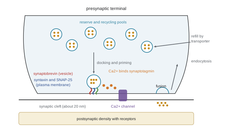
The SNAREs are also the targets of some of the most potent toxins known. Botulinum neurotoxins, produced by Clostridium botulinum, are proteases that cleave SNAP-25, syntaxin or synaptobrevin at cholinergic terminals, blocking acetylcholine release and causing flaccid paralysis; a lethal dose for a human is estimated at around a nanogram per kilogram. Tetanus toxin cleaves synaptobrevin but is transported retrogradely into the spinal cord, where it blocks release from inhibitory interneurons and causes spastic paralysis. The same specificity makes botulinum toxin a medicine: tiny local injections treat dystonia, spasticity, chronic migraine and excessive sweating, as well as reducing wrinkles.
The vesicle cycle
A terminal contains a few hundred vesicles, of which only a small readily releasable pool, perhaps 5 to 10 per active zone, is docked and primed. A recycling pool supports moderate activity, and a larger reserve pool is mobilized only by intense stimulation. After fusion, vesicle membrane is retrieved by endocytosis. Clathrin-mediated endocytosis takes tens of seconds; faster modes, including ultrafast endocytosis discovered by flash-and-freeze electron microscopy in 2013, retrieve membrane within about 100 milliseconds. Whether some vesicles open only briefly through a fusion pore and close again, called kiss-and-run, remains debated. Retrieved vesicles are acidified by a proton pump and refilled by vesicular transporters (VGLUT for glutamate, VGAT for GABA and glycine, VMAT for monoamines, VAChT for acetylcholine). The transporter a neuron expresses largely determines which transmitter it releases.
Short-term plasticity
Synaptic strength changes from moment to moment during repetitive activity. At low-release-probability synapses, residual calcium from one spike adds to the calcium of the next, increasing release: paired-pulse facilitation, lasting tens to hundreds of milliseconds. At high-release-probability synapses, the readily releasable pool depletes quickly and responses depress during a train. Most synapses show a mixture, described by models in which a resource \(x\) is used up by a fraction \(u\) at each spike and recovers with time constant \(\tau_{\text{rec}}\), while \(u\) itself is increased by facilitation. The Tsodyks–Markram model of 1997 captures this with three parameters.
Short-term dynamics act as filters. A depressing synapse responds strongly to the first spike of a burst and to changes in rate, transmitting onsets and novelty; a facilitating synapse responds weakly to isolated spikes and strongly to bursts, acting as a high-pass filter for sustained high-frequency firing. The same axon can make facilitating synapses on one target type and depressing synapses on another: pyramidal cell axons depress onto fast-spiking basket cells but facilitate onto Martinotti cells, so the two inhibitory circuits are recruited at different phases of activity.
# Tsodyks-Markram synapse: depressing vs facilitating responses to a 20 Hz train.
import numpy as np
def train(U, tau_rec, tau_fac, rate=20.0, n=8):
    isi = 1000.0 / rate                 # ms
    x, u = 1.0, U                      # available resources, utilization
    out = []
    for i in range(n):
        if i > 0:
            x = 1 - (1 - x) * np.exp(-isi / tau_rec)      # recovery of resources
            u = U + (u - U) * np.exp(-isi / tau_fac)       # decay of facilitation
            u = u + U * (1 - u)                           # facilitation at the spike
        release = u * x
        out.append(release)
        x -= release
    return np.array(out) / out[0]

dep = train(U=0.6, tau_rec=800.0, tau_fac=10.0)
fac = train(U=0.08, tau_rec=100.0, tau_fac=600.0)
print("spike:          " + " ".join(f"{i+1:5d}" for i in range(8)))
print("depressing:     " + " ".join(f"{v:5.2f}" for v in dep))
print("facilitating: " + " ".join(f"{v:5.2f}" for v in fac))spike: 1 2 3 4 5 6 7 8 depressing: 1.00 0.61 0.18 0.11 0.10 0.10 0.10 0.10 facilitating: 1.00 1.83 2.38 2.73 2.95 3.10 3.22 3.31
Postsynaptic receptors: ionotropic and metabotropic
Transmitters act on two classes of receptor. Ionotropic receptors are ligand-gated ion channels: binding opens a pore within a millisecond, producing a fast postsynaptic current. They include the glutamate receptors (AMPA, NMDA and kainate types, tetramers), the pentameric Cys-loop family (nicotinic acetylcholine receptors, GABA-A, glycine and 5-HT3 receptors) and P2X receptors for ATP. Metabotropic receptors are G-protein-coupled receptors (GPCRs) with seven membrane-spanning helices. Binding activates a heterotrimeric G protein, which acts through second messengers such as cyclic AMP, inositol trisphosphate and diacylglycerol, or directly through its beta-gamma subunits on ion channels. Responses start within tens of milliseconds and can last seconds to minutes, and they can change gene expression over hours. Most transmitters act on both kinds: glutamate on AMPA and NMDA receptors and on metabotropic mGluRs, GABA on GABA-A and GABA-B, acetylcholine on nicotinic and muscarinic receptors.
| Feature | Ionotropic receptor | Metabotropic receptor |
|---|---|---|
| Structure | Ligand-gated channel (tetramer, pentamer or trimer) | Seven-transmembrane GPCR |
| Speed | Under 1 ms to open | Tens of ms to seconds |
| Duration of effect | Milliseconds | Seconds to minutes; gene expression over hours |
| Signaling | Direct ion flow | G proteins and second messengers |
| Amplification | None beyond channel conductance | Large: one receptor activates many G proteins |
| Examples | AMPA, NMDA, GABA-A, nicotinic, glycine | mGluRs, GABA-B, muscarinic, dopamine, opioid receptors |
A synaptic current has its own time course. AMPA receptor currents rise in a few hundred microseconds and decay in a few milliseconds; NMDA receptor currents rise more slowly and decay over 50 to 300 milliseconds, providing a slow component important for temporal integration and plasticity. A convenient description of a synaptic conductance is the alpha function, \(g(t) = g_{\max} (t/\tau) e^{1 - t/\tau}\), which rises to a peak at \(t = \tau\) and then decays. Summing alpha-shaped EPSPs shows how timing determines whether inputs reach threshold.
# Temporal summation of alpha-function EPSPs on a passive membrane.
import numpy as np
dt = 0.1
t = np.arange(0, 120, dt)
tau_syn, tau_m = 2.0, 20.0                 # ms
def epsp(t0, amp=1.0):
    s = np.clip(t - t0, 0, None)
    current = (s / tau_syn) * np.exp(1 - s / tau_syn) * (t >= t0)
    v = np.zeros_like(t)
    for i in range(1, len(t)):               # passive membrane low-pass filter
        v[i] = v[i-1] + dt / tau_m * (-v[i-1] + amp * 4.0 * current[i])
    return v
single = epsp(10)
print(f"single EPSP peak {single.max():.2f} mV at {t[single.argmax()]:.1f} ms")
for isi in (2, 5, 10, 20, 40):
    v = epsp(10) + epsp(10 + isi) + epsp(10 + 2 * isi) + epsp(10 + 3 * isi)
print(f"4 EPSPs, interval {isi:2d} ms: peak {v.max():5.2f} mV")single EPSP peak 0.79 mV at 18.0 ms 4 EPSPs, interval 2 ms: peak 3.02 mV 4 EPSPs, interval 5 ms: peak 2.58 mV 4 EPSPs, interval 10 ms: peak 1.94 mV 4 EPSPs, interval 20 ms: peak 1.30 mV 4 EPSPs, interval 40 ms: peak 0.93 mV
Four EPSPs arriving 2 milliseconds apart summate to nearly four times the single peak, whereas the same four spread 40 milliseconds apart barely summate at all. This is why synchrony among inputs is so effective at driving neurons, and why the membrane time constant defines the window for integration. (In real neurons the nonlinearities of lesson 3 modify this simple picture.)
Electrical synapses
Electrical synapses are gap junctions, clusters of channels formed by connexin proteins (mainly connexin-36 in mammalian neurons) that directly connect the cytoplasm of two cells. Current flows with essentially no delay, in both directions in most cases, and small molecules can pass. Electrical synapses synchronize the firing of coupled neurons, for instance networks of inhibitory interneurons in the cortex and neurons of the inferior olive, and mediate fast escape responses such as the Mauthner cell circuit of fish. They are less flexible than chemical synapses, cannot invert sign or amplify, and are less common in mammals, but they are regulated and can change strength.
Worked problem
Is a change presynaptic or postsynaptic?
After an experimental treatment, the mean EPSP at an invented synapse doubles from 0.8 to 1.6 mV. The failure rate falls from 0.40 to 0.16 and the mean miniature EPSP stays at 0.4 mV. Is the change presynaptic or postsynaptic?
Show solution
- Quantal size q is unchanged at 0.4 mV, so the postsynaptic response to a single vesicle has not changed.
- Quantal content m = mean EPSP / q rises from 2 to 4.
- Using the Poisson failures method, m = −ln(failures): −ln(0.40) ≈ 0.92 before and −ln(0.16) ≈ 1.83 after, also a doubling, consistent with more release.
- The two estimates of m differ in magnitude because p is not small, but both indicate increased release.
Answer: The change is presynaptic: more vesicles are released per action potential, while quantal size is unchanged.
Common mistakes
MistakeAssuming every action potential releases transmitter at every synapse.
InsteadRelease is probabilistic; many central synapses have release probabilities well below 0.5.
MistakeTreating release as proportional to calcium concentration.
InsteadRelease rises roughly with the fourth power of calcium, so small changes in influx have large effects.
MistakeSaying a transmitter is excitatory or inhibitory in itself.
InsteadThe effect depends on the receptor and the ion it passes; acetylcholine excites skeletal muscle but slows the heart.
MistakeConfusing botulinum and tetanus toxins' effects.
InsteadBotulinum blocks release at neuromuscular junctions, causing flaccid paralysis; tetanus blocks spinal inhibitory release, causing spastic paralysis.
MistakeAssuming synaptic strength is fixed between learning episodes.
InsteadShort-term facilitation and depression change strength over milliseconds to seconds during normal activity.
Summary and key terms
- Transmitter is released in quanta; mean response = npq, and failures, means and variances reveal n, p and q.
- Release follows calcium entry within about 0.2 ms and rises roughly with the fourth power of calcium.
- SNARE zippering drives fusion; Munc18 and Munc13 assemble complexes, complexin clamps and synaptotagmin senses calcium.
- Botulinum and tetanus toxins cleave SNAREs; vesicles are recycled by several modes of endocytosis and refilled by specific transporters.
- Short-term facilitation and depression make synapses temporal filters.
- Ionotropic receptors give fast, brief responses; metabotropic GPCRs give slow, amplified, long-lasting ones.
- Electrical synapses through connexin gap junctions couple neurons directly and synchronize them.
- quantum
- The response to the transmitter content of a single vesicle.
- quantal content
- The mean number of vesicles released per action potential.
- release probability
- The probability that a release site releases a vesicle in response to an action potential.
- SNARE complex
- The four-helix bundle of synaptobrevin, syntaxin and SNAP-25 that drives membrane fusion.
- synaptotagmin
- The vesicle calcium sensor that triggers fast synchronous release.
- readily releasable pool
- Docked, primed vesicles available for immediate release.
- paired-pulse facilitation
- An increased response to the second of two closely spaced stimuli.
- synaptic depression
- A decrease in response during repeated stimulation, often from vesicle depletion.
- ionotropic receptor
- A receptor that is itself an ion channel.
- metabotropic receptor
- A G-protein-coupled receptor that acts through intracellular signaling.
Practice problems
Work each problem on paper first, then reveal the answer to check.
A synapse has n = 10 sites, p = 0.2 and q = 0.3 mV. What is the mean EPSP?
Show answer
10 × 0.2 × 0.3 = 0.6 mV.
With a Poisson mean of 0.5 quanta, what fraction of trials fail?
Show answer
e^(−0.5) ≈ 0.61.
If calcium influx falls by 30 percent, by roughly how much does release fall under a fourth-power law?
Show answer
0.7⁴ ≈ 0.24, so release falls to about a quarter.
Which SNARE proteins are on the plasma membrane?
Show answer
Syntaxin-1 and SNAP-25.
Why does a high-release-probability synapse depress during a train?
Show answer
It depletes its readily releasable pool faster than the pool recovers.
Give an example of a transmitter acting on both receptor classes.
Show answer
GABA on GABA-A (ionotropic) and GABA-B (metabotropic), or glutamate on AMPA and mGluRs.
Why do synchronous inputs drive a neuron more effectively than the same inputs spread out?
Show answer
Their EPSPs overlap in time and summate before decaying.
What protein forms neuronal gap junctions in mammals?
Show answer
Mainly connexin-36.
Lesson quiz · 5 questions
Score 60% or more to complete this lesson.
Create a free account to save your progress, take quizzes and earn a certificate.