
BIOL-420 · Lesson 3 of 12 · 26 min
Dendrites, cables and neural integration
A cortical pyramidal neuron receives roughly 10,000 excitatory synapses and a few thousand inhibitory ones, scattered over dendrites that extend hundreds of micrometers from the cell body. Whether the neuron fires depends on how those inputs combine on their way to the axon initial segment. For a long time dendrites were treated as passive wires that simply delivered current to the soma. We now know they filter, attenuate, amplify and even compute. This lesson develops cable theory, the physics of current flow in thin processes, and then shows how voltage-gated channels in dendrites turn a single neuron into something closer to a network of computing subunits.
Why dendrites are cables
A dendrite is a thin cylinder of cytoplasm, a poor conductor, wrapped in membrane that leaks current through open channels. Current injected at one point flows along the core and leaks out through the membrane, so voltage decays with distance, like water leaking from a porous garden hose. Two resistances compete: the axial resistance of the cytoplasm along the cable and the membrane resistance across it. Their balance sets the length constant \(\lambda\), the distance over which a steady voltage falls to \(1/e\), about 37 percent, of its starting value in an infinitely long cable:
where \(R_m\) is the specific membrane resistance (ohm square centimeters), \(R_i\) the specific axial resistance of cytoplasm (ohm centimeters) and \(d\) the diameter. Doubling the diameter increases \(\lambda\) by a factor of the square root of two. With typical values of \(R_m\) = 20,000 Ω cm², \(R_i\) = 150 Ω cm and d = 2 µm, \(\lambda\) is about 0.8 mm. BIOL-350 used the same quantity to explain conduction in axons; here the question is how synaptic signals travel to the soma.
Time matters as well as distance. The membrane time constant \(\tau_m = R_m C_m\), about 20 ms for \(C_m\) = 1 µF/cm², sets how quickly the membrane charges. The full passive cable equation combines both:
where \(V\) is the deviation from resting potential. For steady current injected at one end of an infinite cable, the solution is a simple exponential, \(V(x) = V_0 e^{-x/\lambda}\). Real dendrites are finite and branched. A finite cable that ends in a sealed tip attenuates less than an infinite one, because current cannot escape out of the end, so it piles up; the voltage profile becomes a hyperbolic cosine. The electrotonic length \(L = \ell/\lambda\) measures a dendrite's length in units of its length constant; many neurons are electrotonically compact for steady signals, with L below 1.
# Steady-state voltage along a passive cable: infinite cable vs finite sealed-end cable.
import numpy as np
Rm, Ri, Cm = 20000.0, 150.0, 1.0         # ohm cm^2, ohm cm, uF/cm^2
for d_um in (0.5, 1.0, 2.0, 4.0):
    d = d_um * 1e-4                        # cm
    lam_mm = np.sqrt(Rm * d / (4 * Ri)) * 10
    print(f"diameter {d_um:3.1f} um: lambda = {lam_mm:4.2f} mm")
print("tau_m =", Rm * Cm * 1e-3, "ms")

lam = np.sqrt(Rm * 2e-4 / (4 * Ri)) * 10  # mm, for a 2 um dendrite
ell = 0.6                                  # dendrite length in mm
L = ell / lam
print(f"\n2 um dendrite, length {ell} mm: electrotonic length L = {L:.2f}")
print(" x (mm)   infinite cable   sealed-end cable  (V/V0)")
for x in np.linspace(0, ell, 7):
    inf = np.exp(-x / lam)
    sealed = np.cosh((ell - x) / lam) / np.cosh(ell / lam)
print(f" {x:5.2f} {inf:5.3f} {sealed:5.3f}")diameter 0.5 um: lambda = 0.41 mm diameter 1.0 um: lambda = 0.58 mm diameter 2.0 um: lambda = 0.82 mm diameter 4.0 um: lambda = 1.15 mm tau_m = 20.0 ms 2 um dendrite, length 0.6 mm: electrotonic length L = 0.73 x (mm) infinite cable sealed-end cable (V/V0) 0.00 1.000 1.000 0.10 0.885 0.931 0.20 0.783 0.875 0.30 0.693 0.833 0.40 0.613 0.803 0.50 0.542 0.786 0.60 0.480 0.780
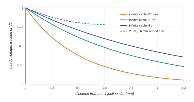
The sealed-end cable keeps far more of its voltage at the tip than the infinite cable predicts, which is why many neurons are electrically compact for slow, steady signals. That does not mean synapses on distant dendrites are as effective as synapses near the soma, for three reasons that follow.
Fast signals attenuate more
Synaptic potentials are brief. A fast excitatory postsynaptic potential (EPSP) rises in a millisecond or two. The membrane capacitance acts as a low-pass filter: high-frequency components leak away as capacitive current before they travel far. An EPSP recorded at its dendritic site may be 10 to 20 millivolts and rise in under a millisecond, while the same event recorded at the soma may be only 0.5 to 1 millivolt, rising over several milliseconds and decaying slowly. Direct dual recordings from dendrite and soma, pioneered by Greg Stuart and Bert Sakmann in the 1990s, confirmed this. The slower somatic waveform means distal inputs have broader time windows for summation, while proximal inputs carry precise timing.
Wilfrid Rall, who developed cable theory for neurons from the late 1950s, showed how to estimate where on a dendrite a synapse lies from the shape of the somatic EPSP: distal inputs rise more slowly and are broader. He also showed that if, at every branch point, the parent diameter raised to the 3/2 power equals the sum of the daughter diameters raised to the 3/2 power, a whole branched tree behaves electrically like a single equivalent cylinder. Few real neurons obey Rall's 3/2 rule exactly, but the idea made analysis possible, and compartmental models later replaced it.
Compartmental models
To simulate realistic neurons, the dendritic tree is divided into short compartments, each small enough to be nearly isopotential, connected by axial resistances. Each compartment has its own membrane capacitance, leak and, if desired, voltage-gated and synaptic conductances. Programs such as NEURON, developed by Michael Hines and Ted Carnevale, solve thousands of coupled equations efficiently, using morphologies reconstructed from real cells. The simplest useful case has just two compartments, a soma and a dendrite, coupled by a conductance.
# Two-compartment neuron: dendrite and soma coupled by an axial conductance.
# A brief synaptic current is injected into the dendrite; compare voltages at both sites.
import numpy as np
dt, T = 0.01, 60.0                    # ms
t = np.arange(0, T, dt)
Cd, Cs = 20.0, 100.0                  # pF (small dendritic compartment, larger soma)
gLd, gLs = 1.0, 5.0                   # nS leak conductances (tau = 20 ms in each)
gc = 2.0                              # nS coupling conductance

def run(gc):
    Vd, Vs = 0.0, 0.0                 # mV relative to rest
    peak_d = peak_s = 0.0
    t_peak_s = 0.0
    for ti in t:
        I_syn = 200.0 * (ti / 0.5) * np.exp(1 - ti / 0.5) if ti > 0 else 0.0   # pA, alpha shape
        dVd = (-gLd * Vd - gc * (Vd - Vs) + I_syn) / Cd
        dVs = (-gLs * Vs - gc * (Vs - Vd)) / Cs
        Vd += dt * dVd
        Vs += dt * dVs
        if Vd > peak_d: peak_d = Vd
        if Vs > peak_s: peak_s, t_peak_s = Vs, ti
    return peak_d, peak_s, t_peak_s

for g in (0.5, 2.0, 10.0):
    pd, ps, tp = run(g)
    print(f"coupling {g:4.1f} nS: dendritic peak {pd:5.2f} mV, somatic peak {ps:5.2f} mV "
f"(ratio {ps/pd:4.2f}), somatic peak time {tp:4.1f} ms")coupling 0.5 nS: dendritic peak 11.59 mV, somatic peak 0.39 mV (ratio 0.03), somatic peak time 16.7 ms coupling 2.0 nS: dendritic peak 10.46 mV, somatic peak 0.96 mV (ratio 0.09), somatic peak time 11.2 ms coupling 10.0 nS: dendritic peak 7.40 mV, somatic peak 1.67 mV (ratio 0.23), somatic peak time 5.5 ms
The model reproduces the experimental pattern: a large, fast dendritic potential becomes a small, delayed somatic one. Stronger coupling, which corresponds to a thicker or shorter dendrite, transfers more of the signal. Even this tiny model is enough to explain why a synapse's location shapes its influence, and adding active channels to the dendritic compartment begins to show the phenomena described next.
Synaptic integration
A neuron sums its inputs in space and time. Spatial summation combines EPSPs arriving at different synapses at the same time; temporal summation combines EPSPs arriving in quick succession at one synapse, which works because each EPSP outlasts the interval between them. Summation is not simply additive. A synaptic conductance drives current proportional to the driving force \((V - E_{\text{syn}})\), so as one input depolarizes the membrane it reduces the driving force for a nearby input; neighboring inputs on the same thin branch therefore sum sublinearly, while inputs on separate branches sum nearly linearly.
Inhibition does not just subtract. A GABA-A synapse whose reversal potential is close to rest produces little voltage change on its own, yet it opens a conductance that shunts current, short-circuiting nearby excitatory inputs; this is shunting inhibition. Its effect is greatest when it sits on the path between the excitatory inputs and the soma, which is why many inhibitory interneurons target the soma and axon initial segment (basket cells and chandelier cells) where they can veto output, while others target distal dendrites (Martinotti and neurogliaform cells) to control specific input streams.
Active dendrites
Dendrites contain voltage-gated sodium, calcium, potassium and HCN channels, and NMDA receptors. These make dendrites active participants rather than passive cables:
Back-propagating action potentials. When a neuron fires, the spike travels not only down the axon but also back into the dendrites, carried by dendritic sodium channels. Back-propagation tells synapses that the neuron has fired, which is essential for spike-timing-dependent plasticity (lesson 6). A-type potassium channels, more dense in distal dendrites, limit how far spikes back-propagate.
Dendritic spikes. Strong, clustered input to a dendritic branch can trigger local regenerative events: sodium spikes lasting a millisecond or so, calcium spikes lasting tens of milliseconds, and NMDA spikes, plateau potentials of 50 to 100 milliseconds produced when glutamate-bound NMDA receptors are relieved of their magnesium block by depolarization. In layer 5 pyramidal neurons, Matthew Larkum and colleagues showed in 1999 that a back-propagating spike coinciding with distal input triggers a calcium spike near the apical tuft that produces a burst of axonal spikes, a mechanism called back-propagation-activated calcium spike (BAC) firing. It lets a neuron detect coincidence between feedforward input to its basal dendrites and feedback input from higher areas to its tuft.
Location-dependent scaling. In hippocampal CA1 neurons, the conductance of distal synapses is larger than that of proximal ones, partly compensating for attenuation, so that inputs at different distances have more similar effects at the soma. HCN channels, which increase in density toward the distal dendrites, shorten the time course of distal EPSPs and reduce the location dependence of temporal summation.
Because each thin branch can produce its own nonlinear response, Bartlett Mel and Panayiota Poirazi proposed in 2003 that a pyramidal neuron can be modeled as a two-layer network: each branch applies a sigmoid-like nonlinearity to its inputs, and the soma sums the branch outputs. In 2021 a study by Beniaguev, Segev and London trained a deep artificial neural network to mimic a detailed layer 5 pyramidal cell model and needed five to eight layers when NMDA receptors were included, a striking measure of the computational capacity of a single neuron (contrast with the simple units of artificial networks in CMPUT-466). In human cortex, recordings from tissue removed during epilepsy surgery revealed dendritic calcium spikes in layer 2/3 neurons that are largest for intermediate inputs, allowing a single neuron to compute an exclusive-or function, something a single unit in a simple artificial network cannot do.
Spines as compartments
Dendritic spines have a head of about 0.5 to 1 µm connected to the dendrite by a thin neck 0.1 to 0.2 µm across. The neck restricts diffusion of calcium and other signals, so each spine is a biochemical compartment where plasticity can be confined to one synapse. Whether the neck also isolates the spine electrically is debated; estimates of neck resistance range from tens to hundreds of megaohms, enough in some cases to amplify the local depolarization in the spine head and boost NMDA receptor activation. Spines change shape with activity, enlarging during long-term potentiation and shrinking during depression, and their numbers are altered in several conditions, including fragile X syndrome and schizophrenia.
| Property | Proximal input | Distal input |
|---|---|---|
| Somatic EPSP amplitude | Larger | Smaller, unless compensated |
| Somatic EPSP time course | Fast rise and decay | Slow rise, broad |
| Temporal precision | High | Lower |
| Ability to trigger local dendritic spikes | Low (thick dendrite) | High (thin branches, high input resistance) |
| Typical sources in cortex | Local and thalamic input to basal dendrites | Feedback from higher areas to the apical tuft |
From integration to output
After all the filtering, summation and local amplification, the axon initial segment converts the net current into spikes. The neuron's output is a spike train, and information can be carried by firing rate, by the precise timing of spikes relative to stimuli or to network oscillations, or by bursts. In many systems firing rate dominates, but the auditory brainstem uses microsecond timing (lesson 8), and hippocampal place cells encode position partly by the phase at which they fire relative to the theta rhythm (lesson 10). The passive and active properties of dendrites thus determine not only whether a neuron fires but what its spikes mean.
Worked problem
Will a distal synapse be heard at the soma?
An invented thin dendrite (0.8 µm diameter, Rm = 20,000 Ω cm², Ri = 200 Ω cm) receives a synapse 400 µm from the soma. Treating the dendrite as an infinite cable for a steady signal, what fraction of the local depolarization reaches the soma? How would the answer change for a brief EPSP?
Show solution
- λ = √(Rm d / 4Ri) = √(20,000 × 0.8 × 10⁻⁴ / 800) cm = √0.002 cm ≈ 0.045 cm = 0.45 mm.
- Steady attenuation over 0.4 mm: e^(−0.4/0.45) = e^(−0.89) ≈ 0.41.
- A sealed end beyond the synapse would raise this somewhat, but a brief EPSP attenuates much more because the membrane capacitance filters high frequencies.
- In practice the somatic EPSP might be only a few percent of the local amplitude, unless active conductances or larger synaptic conductance compensate.
Answer: About 40 percent for a steady signal, but much less for a fast EPSP, which is why distal synapses often rely on dendritic amplification or synchrony.
Common mistakes
MistakeAssuming EPSPs from all synapses arrive at the soma with equal size.
InsteadDistal EPSPs are attenuated and slowed by cable filtering unless compensated.
MistakeUsing the steady-state length constant to predict attenuation of fast EPSPs.
InsteadFast signals attenuate more because capacitance filters high frequencies.
MistakeThinking inhibition works only by hyperpolarizing the membrane.
InsteadShunting inhibition reduces the effect of excitation by increasing conductance, even with little voltage change.
MistakeTreating dendrites as passive wires.
InsteadDendritic sodium, calcium and NMDA spikes and back-propagating action potentials make them active.
MistakeSumming EPSPs linearly in all cases.
InsteadInputs close together on one branch sum sublinearly through reduced driving force, or supralinearly if they trigger a dendritic spike.
Summary and key terms
- Dendrites behave as leaky cables; λ = √(Rm d / 4Ri) and τm = RmCm set spatial and temporal decay.
- Sealed-end finite cables attenuate steady signals less than infinite ones, but fast EPSPs are strongly filtered.
- Compartmental models divide neurons into coupled isopotential pieces; even two compartments reproduce dendritic attenuation and slowing.
- Integration is nonlinear: driving force effects, shunting inhibition and inhibitory placement shape output.
- Active dendrites support back-propagating spikes, local sodium, calcium and NMDA spikes, and BAC firing.
- Single neurons can perform computations comparable to multi-layer networks; spines compartmentalize plasticity.
- length constant
- The distance over which a steady voltage decays to 1/e in an infinite passive cable.
- membrane time constant
- RmCm, the time for the membrane to charge to about 63 percent of its final voltage.
- electrotonic length
- A cable's physical length divided by its length constant.
- compartmental model
- A neuron model built from coupled, nearly isopotential compartments.
- spatial summation
- Combination of inputs arriving at different synapses at about the same time.
- temporal summation
- Combination of successive inputs at one synapse that overlap in time.
- shunting inhibition
- Inhibition that reduces excitation by increasing membrane conductance.
- back-propagating action potential
- An action potential that spreads from the axon initial segment back into the dendrites.
- NMDA spike
- A dendritic plateau potential produced by regenerative NMDA receptor activation.
- BAC firing
- A burst triggered when a back-propagating spike coincides with distal dendritic input.
Practice problems
Work each problem on paper first, then reveal the answer to check.
By what factor does λ change if dendrite diameter is quadrupled?
Show answer
It doubles, because λ is proportional to the square root of diameter.
Why does a sealed-end cable attenuate less than an infinite cable?
Show answer
Current cannot leave through the end, so it accumulates and raises voltage along the cable.
A somatic EPSP rises slowly and is broad. Where was the synapse probably located?
Show answer
On a distal dendrite.
What is the advantage of placing inhibitory synapses on the axon initial segment?
Show answer
They can veto spike generation regardless of where excitation arrived.
What relieves the magnesium block of NMDA receptors during an NMDA spike?
Show answer
Depolarization of the dendritic branch by clustered excitatory input.
Why are back-propagating action potentials important for learning?
Show answer
They signal to synapses that the neuron has fired, enabling timing-dependent plasticity.
State Rall's 3/2 rule.
Show answer
At each branch point, the parent diameter to the 3/2 power equals the sum of the daughter diameters to the 3/2 power.
What does BAC firing allow a layer 5 neuron to detect?
Show answer
Coincidence between basal (feedforward) input causing a spike and apical (feedback) input to the tuft.
Lesson quiz · 5 questions
Score 60% or more to complete this lesson.
Create a free account to save your progress, take quizzes and earn a certificate.