Small populations and population viability

Once a population has been reduced to a small size, new dangers appear that have little to do with the original cause of decline. Chance events in births and deaths, fluctuations in the environment, the loss of genetic variation and difficulties in finding mates can all push a small population toward extinction, even if the threat that reduced it has been removed. This lesson examines these small-population processes, the idea of a minimum viable population, and population viability analysis (PVA), the main quantitative tool conservation biologists use to estimate extinction risk and compare management options. BIOL-208 introduced demographic stochasticity and matrix models, and BIOL-322 covered genetic drift, effective population size, inbreeding depression and genetic rescue; this lesson builds on both without repeating them.

Two paradigms

In 1994 the Australian ecologist Graeme Caughley argued that conservation biology had developed along two largely separate lines. The small-population paradigm studies the consequences of smallness itself: demographic and environmental stochasticity, genetic deterioration and Allee effects. It is rich in theory but, Caughley argued, had rarely explained why particular populations became small in the first place. The declining-population paradigm studies the causes of decline, such as habitat loss, overharvesting or introduced predators, and how to detect and reverse them. It is practical but less theoretical. Caughley's point was that a population is usually driven to small size by a deterministic cause, and that conservation must first diagnose and remove that cause; only then do the risks of smallness become the main concern. Modern conservation integrates both paradigms. A recovery plan must stop the decline and also manage the risks faced by the small population that remains.

Demographic stochasticity

Every individual either survives or dies and either reproduces or does not, and these outcomes are partly matters of chance. In a large population, the proportion surviving each year closely matches the average survival rate, but in a small population chance fluctuations can be large. If each of ten animals has a 70 percent chance of surviving a year, the expected number of survivors is seven, but there is about a 15 percent chance that five or fewer will survive. Chance also affects the sex ratio: a population of four birds may by bad luck consist entirely of males. The last six dusky seaside sparrows, a subspecies of the Florida coast, were all males when they were taken into captivity in 1979 and 1980; the subspecies was declared extinct when the last one died in 1987. Demographic stochasticity is important mainly in populations of fewer than a few dozen to a hundred individuals, depending on the species.

Environmental stochasticity and catastrophes

Environmental stochasticity is variation in birth and death rates caused by fluctuations in weather, food supply, predators or disease that affect all individuals in a population together. Unlike demographic stochasticity, it does not become less important as populations grow, because a bad year affects a large population as much as a small one, proportionally. Environmental variation also reduces the long-run growth rate of a population. If a population grows by a factor \(\lambda_t\) in year \(t\), its size after many years depends on the product of the yearly factors, and the long-run growth rate is the geometric mean, not the arithmetic mean, of those factors. For small fluctuations the long-run growth rate on a logarithmic scale is approximately

where \(\bar{r}\) is the average yearly growth rate on a logarithmic scale and \(\sigma^2\) is its variance. A population whose average year is slightly positive can therefore decline in the long run if its growth rate is variable enough. For example, a population that grows by 50 percent in good years and shrinks by 40 percent in bad years, with equal frequency, has an arithmetic mean growth factor of 1.05 but a geometric mean of \(\sqrt{1.5 \times 0.6} \approx 0.95\), and it will decline.

Catastrophes are extreme environmental events, such as hurricanes, severe winters, droughts, oil spills or disease outbreaks, that cause sudden large losses. Even a large population confined to a small area can be eliminated by a single catastrophe. Florida's Key deer, the Laysan duck of the Hawaiian Islands and many island species are exposed to storms that could affect their entire range at once. The standard defense against catastrophes is to spread the risk by maintaining several populations in different places, so that a single event cannot affect all of them. This principle of redundancy appears in many recovery plans.

Allee effects

In 1931 the American ecologist Warder Clyde Allee described how individuals of some species do better when they are in groups than when they are alone. When individual fitness declines at low population density, the population is said to experience an Allee effect. Mechanisms include difficulty in finding mates, as in sparse populations of sea urchins or abalone that release eggs and sperm into the water; reduced cooperative defense against predators, as in schooling fish and colonial seabirds; reduced efficiency of cooperative hunting, as in African wild dogs; and reduced pollination of sparse plants. A component Allee effect is a decline in one component of fitness, such as mating success, at low density. A demographic Allee effect occurs when the overall per capita growth rate of the population declines at low density.

A strong Allee effect creates a threshold population size, sometimes called the Allee threshold, below which the population declines toward extinction. One simple model adds a threshold \(A\) to logistic growth:

For populations between \(A\) and \(K\) growth is positive; below \(A\) it is negative. Strong Allee effects explain why some heavily exploited populations, such as certain fish stocks and abalone, have failed to recover even after harvesting stopped, and why reintroductions often need to release animals in groups rather than singly.

Genetic threats in brief

BIOL-322 showed that small populations lose genetic variation by drift at a rate of about \(1/(2N_e)\) per generation, where \(N_e\) is the effective population size, and that inbreeding in small populations reduces fitness through inbreeding depression. Small populations can also accumulate mildly harmful mutations that selection is too weak to remove, a process sometimes called mutational meltdown. The Florida panther, whose small population showed kinked tails, heart defects and poor sperm quality before eight female pumas from Texas were released in 1995, illustrates both the danger and the remedy of genetic rescue. For this lesson the key point is that genetic and demographic processes interact: inbreeding lowers survival and reproduction, which reduces population size, which increases drift and inbreeding further.

The extinction vortex

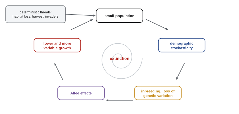
In 1986 Michael Gilpin and Michael Soulé described how these processes can reinforce one another in a downward spiral they called the extinction vortex. A population that becomes small experiences more demographic stochasticity, more inbreeding and loss of genetic variation, and possibly Allee effects; these reduce its growth rate and increase its variability, making it smaller still, which strengthens the same processes. A study by William Fagan and Elizabeth Holmes in 2006, which analyzed time series from ten vertebrate populations that went extinct, found the signature of the vortex: the rate of decline and the variability of population growth both increased as the populations approached extinction. The practical implication is that intervention is easier and cheaper early, before the vortex takes hold.

Minimum viable populations

In 1981 Mark Shaffer defined a minimum viable population (MVP) as the smallest isolated population that has a 99 percent chance of persisting for 1,000 years despite demographic, environmental and genetic stochasticity and natural catastrophes. The definition highlights that viability is a probability over a time horizon, not a fixed number. Early rules of thumb, such as the 50/500 rule proposed by Ian Franklin and Otto Frankel in 1980, suggested that an effective population size of 50 avoids short-term inbreeding depression and 500 retains long-term evolutionary potential; later work suggested that the long-term figure should be higher, perhaps 1,000 or more. A 2007 meta-analysis by Lochran Traill and colleagues estimated MVPs for 212 species and found a median of about 4,000 adults, with wide variation among species. Because MVPs depend on life history, environmental variability, the time horizon and the acceptable level of risk, most conservation biologists now argue that no single number applies across species and that viability must be estimated case by case.

Population viability analysis

Population viability analysis is the use of quantitative models to estimate the probability that a population will persist for a given time, or fall below a given size, under specified conditions. A PVA typically requires estimates of survival and fecundity for each age or stage class, their variation from year to year, density dependence, carrying capacity, the frequency and severity of catastrophes, and sometimes genetic effects and dispersal among subpopulations. The model is run many times with random variation, each run producing one possible future, and the proportion of runs in which the population falls below a quasi-extinction threshold estimates the risk. Quasi-extinction thresholds, such as 20 or 50 individuals, are used because the dynamics of extremely small populations are poorly known and because managers need warning well before the last individual dies.

import numpy as np
rng = np.random.default_rng(367)
# A simple stochastic PVA for an invented species (adult females only, annual census).
# Demographic stochasticity: binomial survival and Poisson births; environmental stochasticity:
# good and bad years shift survival; Allee effect: breeding success falls when females are scarce.
S_MEAN, S_SD, F_MEAN, K, ALLEE = 0.80, 0.12, 0.45, 300, 10
def one_run(n0, years=100, threshold=10, allee=True):
    n = n0
    for _ in range(years):
        s = min(max(rng.normal(S_MEAN, S_SD), 0.0), 1.0)    # environmental variation in survival
        survivors = rng.binomial(n, s)                       # demographic chance in survival
        f = max(F_MEAN * (1 - survivors / K), 0.0)           # density dependence
        if allee:
            f *= survivors / (survivors + ALLEE)             # mate-finding Allee effect
        births = rng.poisson(f * survivors)                  # daughters born to surviving females
        n = min(survivors + births, K)
        if n < threshold:
            return True
    return False
RUNS = 1000
for n0 in (20, 40, 80, 160):
    risk = sum(one_run(n0) for _ in range(RUNS)) / RUNS
    print(f"start with {n0:3d} females: probability of falling below 10 within 100 years = {risk:.2f}")
risk = sum(one_run(40, allee=False) for _ in range(RUNS)) / RUNS
print(f"start with  40 females, no Allee effect: {risk:.2f}")

start with  20 females: probability of falling below 10 within 100 years = 0.69
start with  40 females: probability of falling below 10 within 100 years = 0.29
start with  80 females: probability of falling below 10 within 100 years = 0.12
start with 160 females: probability of falling below 10 within 100 years = 0.08
start with  40 females, no Allee effect: 0.00

The simulation shows how quasi-extinction risk falls steeply as the starting population grows, and how much an Allee effect raises the risk for small populations. With the parameters chosen, a population of a few dozen females grows slowly on average, yet many runs started from small sizes still fall below the threshold through runs of bad years and chance losses early on. Without the Allee effect, the same population of 40 females almost never falls below the threshold, because its growth rate at low density is much higher; the Allee effect turns a comfortable margin into a serious risk. A real PVA would be built from field estimates with their uncertainty, would include age structure and catastrophes, and would explore how sensitive the results are to each parameter.

What PVA is good for

PVA has been criticized because its absolute predictions are uncertain: estimates of extinction probability depend on parameters that are often poorly known, especially variances and the shape of density dependence, and small errors can produce large differences in predicted risk over long horizons. A widely cited test by Barry Brook and colleagues in 2000, however, compared PVA predictions for 21 long-term studies with what actually happened and found that, overall, the predictions were surprisingly accurate and unbiased. Most practitioners agree that PVA is most useful for comparing management options, ranking threats and identifying which vital rates most influence persistence, rather than for producing precise absolute probabilities. A PVA might show, for example, that improving adult survival by five percent reduces extinction risk more than doubling the number of young produced, directing effort toward reducing adult mortality. The software package Vortex, developed by Robert Lacy and used in many recovery programs, includes genetic as well as demographic processes.

PVAs also make assumptions explicit. When stakeholders disagree about whether a population is at risk, building a model forces them to state what they believe about survival, reproduction and threats, and to see how those beliefs translate into outcomes. This makes PVA valuable in structured decision making, discussed in lesson 12.

Small populations in Canada and the United States

Several North American species illustrate small-population problems. The North Atlantic right whale, which feeds in the Gulf of St. Lawrence and calves off the southeastern United States, numbered fewer than 400 individuals in recent estimates, with deaths from ship strikes and entanglement in fishing gear exceeding births in several years; both countries have imposed vessel speed limits and fishery closures in areas where whales are present. The southern resident killer whales of the Salish Sea number fewer than 80 and face shortages of their main prey, Chinook salmon, as well as noise and pollution. The Vancouver Island marmot fell to fewer than 30 animals in the wild in the early 2000s, and its recovery through captive breeding is discussed in lesson 10. In each case, managers must reduce the original threats while managing the extra risks of small size.