Threats I: habitat loss, fragmentation and invasive species

E. O. Wilson summarized the main threats to biodiversity with the acronym HIPPO: habitat destruction, invasive species, pollution, human population and its consumption, and overharvesting. The order roughly reflects their importance, and the first two dominate for most groups of species. This lesson examines habitat loss, the fragmentation of what remains, and the spread of invasive species, with tools for estimating their effects. Lesson 5 covers overexploitation, pollution, disease and climate change. In reality the threats rarely act alone; a species in decline usually faces several at once, and their combined effect can be greater than the sum of their parts.

Habitat loss: the leading threat

For most threatened species on the IUCN Red List, the leading threat is loss or degradation of habitat, and agriculture is the largest single cause. About a third of Earth's ice-free land is now used for crops or pasture. Forests once covered about half of the land area that could support them; roughly a third of that forest has been cleared, most of it in the past three centuries, and tropical deforestation continues at millions of hectares a year. Grasslands and wetlands have been converted even more completely in some regions because they are flat, fertile and easy to plow or drain.

In the United States, roughly half of the wetlands that existed in the contiguous states in the 1780s had been lost by the 1980s, according to a widely cited analysis by Thomas Dahl of the Fish and Wildlife Service; losses exceeded 80 percent in some states such as California, Ohio and Iowa. Tallgrass prairie, which once covered much of the Midwest, survives on only a few percent of its original area, and the longleaf pine forests of the Southeast have been reduced to a few percent of their former extent. In the West, sagebrush steppe is being lost to conversion, energy development, invasive grasses and fire.

Habitat loss is not only outright conversion. Degradation reduces the quality of habitat without destroying it: selective logging that removes old trees with cavities, overgrazing that changes plant communities, fire suppression that allows shrubs to invade grasslands, and drainage that lowers the water table of a fen. Degraded habitat may support some species while losing those with specialized needs, and it may become a sink, where reproduction does not keep up with mortality, a concept introduced in BIOL-208.

Predicting extinctions from habitat loss

The species–area relationship described in lesson 2 can be used in reverse to estimate how many species a region will eventually lose when its habitat shrinks. If the original area \(A_0\) held \(S_0\) species and only \(A_1\) remains, then the expected number of species that will persist is

With \(z = 0.25\), losing 90 percent of a habitat would be expected to eliminate about 44 percent of the species restricted to it, since \(0.1^{0.25} \approx 0.56\). This method has been used to estimate global extinction rates from deforestation. It has also been criticized for overestimating losses, because species–area curves built by adding area are not exactly reversed when area is removed: a species must lose all of its individuals to go extinct, whereas it is counted as present as soon as one individual appears. Fangliang He and Stephen Hubbell argued in 2011 that this asymmetry can make the simple method overestimate extinctions, sometimes greatly. Other refinements account for the fact that some species survive in the human-modified matrix around remnants, using the countryside species–area relationship proposed by Henrique Pereira and Gretchen Daily. Despite these debates, the method gives useful first estimates, and the number it predicts is best thought of as eventual losses, much of it an extinction debt that will be paid over decades.

# Expected species loss from habitat loss with the species-area relationship, S1/S0 = (A1/A0)^z.
# Invented example: a region with 240 species restricted to native grassland.
S0 = 240
for remaining in (0.75, 0.50, 0.25, 0.10, 0.05):
    row = []
    for z in (0.15, 0.25, 0.35):
        lost = S0 * (1 - remaining ** z)
        row.append(f"z={z:.2f}: {lost:5.1f}")
    print(f"{remaining:5.0%} habitat left -> species eventually lost  " + "   ".join(row))
# Countryside version: the converted land still supports some species at a fraction h of native habitat value.
h = 0.2
for remaining in (0.25, 0.10):
    effective = remaining + h * (1 - remaining)
    print(f"countryside model, h = {h}, {remaining:.0%} left: about {S0 * (1 - effective ** 0.25):.0f} lost instead of {S0 * (1 - remaining ** 0.25):.0f}")

  75% habitat left -> species eventually lost  z=0.15:  10.1   z=0.25:  16.7   z=0.35:  23.0
  50% habitat left -> species eventually lost  z=0.15:  23.7   z=0.25:  38.2   z=0.35:  51.7
  25% habitat left -> species eventually lost  z=0.15:  45.1   z=0.25:  70.3   z=0.35:  92.3
  10% habitat left -> species eventually lost  z=0.15:  70.1   z=0.25: 105.0   z=0.35: 132.8
   5% habitat left -> species eventually lost  z=0.15:  86.9   z=0.25: 126.5   z=0.35: 155.9
countryside model, h = 0.2, 25% left: about 49 lost instead of 70
countryside model, h = 0.2, 10% left: about 65 lost instead of 105

The output shows two important points. First, losses rise slowly at first and then steeply: losing a quarter of the habitat costs relatively few species, but losing the last few percent costs many. This is one reason conservation biologists argue that the remaining fragments of heavily converted ecosystems, such as tallgrass prairie, are especially valuable. Second, the predictions depend strongly on assumptions. Changing z from 0.15 to 0.35, or allowing modified land to support some species, changes the predicted loss by tens of species. Good practice is to report a range, not a single number.

Fragmentation

Habitat loss is usually accompanied by fragmentation, the breaking of continuous habitat into smaller, more isolated pieces separated by a matrix of different land use. Fragmentation has several components: a reduction in total habitat, a decrease in the size of patches, an increase in the number of patches, an increase in isolation, and an increase in the amount of edge relative to interior. These components often occur together but have different effects. Lenore Fahrig has argued, based on reviews published in 2003 and 2017, that most of the negative effects attributed to fragmentation are really effects of habitat loss, and that when total habitat amount is held constant, fragmentation per se often has weak or even positive effects. Others have responded that experiments and long-term studies, such as the Biological Dynamics of Forest Fragments Project in the Amazon, show strong negative effects of fragmentation, especially through edge effects and isolation. The debate has sharpened thinking: managers need to know whether to prioritize the total amount of habitat or its configuration, and the answer may differ among species.

Edge effects

The boundary between a habitat patch and the surrounding matrix is a zone of altered conditions called an edge. Forest edges are brighter, warmer, drier and windier than forest interiors, and these physical changes can extend tens of meters into the forest, with some effects reaching 100 meters or more. Biological edge effects can extend further. In North America, nest predation by raccoons, crows, jays and domestic cats is often higher near edges, and the brown-headed cowbird, a brood parasite that lays its eggs in the nests of other birds and forages in open land, parasitizes forest songbirds most heavily near edges. Studies in the Midwest in the 1980s and 1990s found that some songbirds in small, fragmented woodlots produced too few young to sustain their populations; the woodlots acted as sinks, and the populations persisted only because of immigration from larger forests.

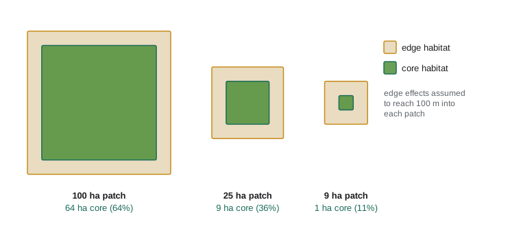
Because edge effects penetrate a fixed distance, small patches can be all edge and no interior. A square patch of side \(L\) with edge effects reaching a depth \(d\) has a core area of \((L - 2d)^2\), which falls to zero when \(L \le 2d\). A 100-hectare square, 1,000 meters on a side, with an edge depth of 100 meters has a core area of 64 hectares, 64 percent of the total; a 9-hectare square with the same edge depth has a core of only 1 hectare, about 11 percent. Shape matters as well as size: long, thin or irregular patches have more edge per unit area than compact ones.

Roads and linear features

Roads fragment habitat in a particularly damaging way. They kill animals directly: road mortality is a major threat to turtles, snakes, amphibians and some large mammals, and it is estimated to kill millions of vertebrates a year in North America. They act as barriers that some species refuse to cross, dividing populations genetically. They bring noise, light, pollution and invasive plants along their verges, and they provide access for hunters, poachers, off-road vehicles and further development. Richard Forman and colleagues developed the field of road ecology in the 1990s and 2000s and estimated that the ecological effects of roads in the United States extend over about a fifth of the land area.

Linear features from resource development have similar effects. In the boreal forest, seismic lines cut for oil and gas exploration, pipelines, power lines and logging roads have created dense networks in some regions. Boreal woodland caribou are threatened largely because these features, together with cutblocks and fire, create young forest that supports moose and deer, which in turn support more wolves; the linear features also let wolves travel faster and hunt more efficiently. The federal recovery strategy for boreal caribou, published in 2012 and amended since, set a threshold of at least 65 percent undisturbed habitat in a caribou range to give a measurable probability, about 60 percent, that the local population will be self-sustaining. Many ranges in Alberta and British Columbia are far below this threshold.

Invasive species

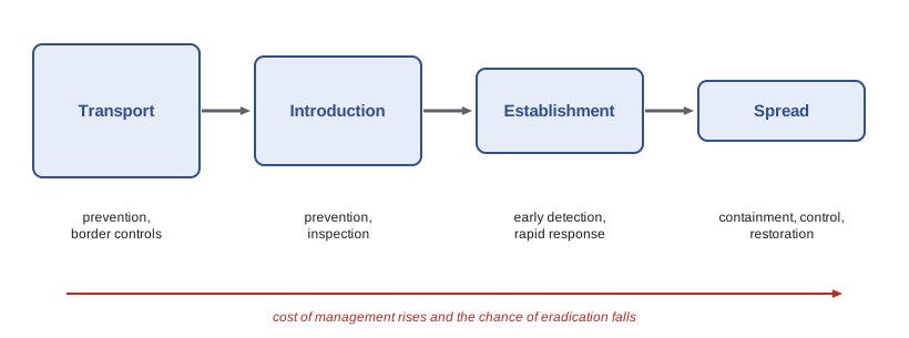
An invasive species is a non-native species that establishes, spreads and causes ecological or economic harm in a region outside its native range. Not every introduced species becomes invasive. Mark Williamson's tens rule, proposed in the 1990s, suggested that roughly one in ten species imported to a region appears in the wild, one in ten of those establishes a self-sustaining population, and one in ten of those becomes a pest. The proportions vary widely among groups, but the rule captures the idea that invasion is a sequence of filters. The stages of an invasion are transport, introduction, establishment and spread, and different management actions apply at each stage.

In 2023 IPBES published a thematic assessment of invasive alien species. It reported that more than 37,000 alien species have been established by human activities around the world, with about 200 new ones recorded each year; that invasive species were a major factor in about 60 percent of recorded global animal and plant extinctions and the only factor in 16 percent; and that the global economic cost of biological invasions exceeded 423 billion US dollars a year in 2019, having quadrupled every decade since 1970. Island species are particularly vulnerable: introduced rats, cats, goats and pigs, along with diseases, have caused most recorded bird extinctions on islands such as Hawaii, Guam and New Zealand.

Several hypotheses explain why some introduced species become so successful. The enemy release hypothesis proposes that species escape the predators, parasites and diseases that controlled them in their native range. The propagule pressure hypothesis notes that species introduced in large numbers, repeatedly, are more likely to establish. Novel weapons, such as chemicals released by some invasive plants that suppress native plants, give some invaders an advantage. And disturbed habitats, where native communities have already been weakened, are often easier to invade.

North America has many well-known invaders. Zebra mussels and the closely related quagga mussels arrived in the Great Lakes in ballast water from Europe in the late 1980s; they filter enormous volumes of water, have caused the collapse of native freshwater mussels in many areas, foul water intakes and have spread into many inland lakes on trailered boats. The emerald ash borer, a beetle from Asia detected near Detroit and Windsor in 2002, has killed hundreds of millions of ash trees in the eastern half of the continent; black ash, which is culturally important to many Indigenous peoples for basket making, is among the species at risk. Invasive carps from Asia, including bighead and silver carp, spread up the Mississippi River system after escaping from aquaculture facilities, and electric barriers in the Chicago Sanitary and Ship Canal are designed to prevent them reaching the Great Lakes. Burmese pythons in the Everglades, feral pigs across the southern United States, European green crabs on both coasts, and cheatgrass in the western sagebrush steppe, which increases the frequency of fire, are further examples.

Prevention is far cheaper than control. Inspection of ballast water under international rules that came into force in 2017, restrictions on the trade in live animals and plants, clean-drain-dry programs for boats and controls on moving firewood all aim to stop invasions at the first stages. Early detection and rapid response can sometimes eradicate a new population before it spreads. Once a species is widespread, eradication is usually impossible except on islands, where removing rats, cats or goats has allowed seabirds and other species to recover dramatically; hundreds of island eradications have now been carried out around the world. Biological control, the release of a natural enemy from the invader's native range, can work well, as with beetles that have controlled purple loosestrife in some wetlands, but it carries the risk that the control agent will attack native species, as happened with some early introductions, and is now subject to careful testing.