Microbial ecology and the microbiome

Microbes rarely live alone. In soil, water, sediments and the bodies of plants and animals they form communities of hundreds to thousands of species that compete, cooperate, exchange genes and signals and together carry out processes no single species could. Microbial ecology asks who is there, what they are doing and how communities are assembled and maintained. For most of the twentieth century these questions were nearly impossible to answer because most microbes could not be cultured (lesson 1). Sequencing has changed that. This lesson describes microbial habitats and community behaviors such as biofilm formation and quorum sensing, explains how communities are surveyed with 16S rRNA sequencing and metagenomics and how the results are analyzed, and then looks critically at the human microbiome. BIOL-208 covered general ecological principles, including diversity indices and nutrient cycles; here they are applied to microbial data.

Microbial habitats

Microbial habitats are defined at the scale of the microbe, the microenvironment, which may be only a few hundred micrometers across. A single soil aggregate can have an oxygenated surface and an anoxic core, so aerobes and anaerobes live millimeters apart. Soil is one of the most diverse habitats known, with roughly 10⁹ cells and thousands of species per gram, dominated by groups such as Acidobacteriota, Actinomycetota, Pseudomonadota and Verrucomicrobiota, together with ammonia-oxidizing archaea and fungi. Soil microbes decompose organic matter, cycle nitrogen and phosphorus, form symbioses with plant roots and produce most of our antibiotics.

The open ocean is dominated by tiny, streamlined cells adapted to very low nutrient levels. The cyanobacterium Prochlorococcus, about 0.6 µm across and discovered only in 1988, is probably the most abundant photosynthetic organism on Earth and carries out a substantial fraction of ocean primary production. The heterotrophic SAR11 clade (Pelagibacter) is the most abundant group of marine bacteria, with very small genomes and cells specialized to take up scarce dissolved organic compounds. Marine viruses kill a large share of these cells daily, releasing dissolved organic matter in what is called the viral shunt. In the deep subsurface, microbes live kilometers below the surface in rock and sediment, metabolizing extremely slowly on hydrogen from rock–water reactions or on ancient buried organic matter; the deep biosphere may contain a substantial fraction of all prokaryotic cells.

Extreme environments host specialists described in earlier lessons: thermophiles and hyperthermophiles in hot springs and hydrothermal vents, halophiles in salt lakes and evaporation ponds, acidophiles in acid mine drainage and psychrophiles in sea ice and permafrost. Hydrothermal vents support whole ecosystems based on chemolithotrophy, where tube worms and clams depend on symbiotic sulfur-oxidizing bacteria rather than on sunlight.

Biofilms

Most microbes in nature live in biofilms, communities attached to surfaces and embedded in a self-produced matrix of extracellular polymeric substances: polysaccharides, proteins, DNA and lipids. A biofilm forms in stages. Free-swimming cells attach reversibly to a surface, often one already coated with organic molecules; they then attach irreversibly with adhesins and pili, multiply to form microcolonies, secrete the matrix and develop a three-dimensional structure with water channels; finally some cells disperse to colonize new sites. Dental plaque, the slime in drains and on river stones, the films inside water pipes and the mats in hot springs are all biofilms.

Biofilm life has advantages. The matrix protects cells against drying, grazing by protozoa, the host immune system, disinfectants and antibiotics; the close packing favors cooperation, metabolic cross-feeding and horizontal gene transfer; and gradients of oxygen and nutrients create niches for many species. Cells deep in a biofilm grow slowly and include many persisters (lesson 5), and the matrix slows the penetration of some antimicrobials. As a result, bacteria in biofilms can tolerate antibiotic concentrations 100 to 1,000 times higher than the MIC of the same strain growing freely. Biofilms on medical devices, such as catheters, artificial joints and heart valves, cause persistent infections that often require removal of the device, and the Pseudomonas aeruginosa biofilms in the lungs of people with cystic fibrosis are notoriously hard to eradicate. Industry spends large sums controlling biofilms that foul ship hulls, clog heat exchangers and harbor Listeria in food plants (lesson 11).

Quorum sensing

Many bacteria coordinate their behavior according to population density by quorum sensing. Each cell releases a small signal molecule, called an autoinducer, at a low rate. At low density the signal diffuses away; as density rises, it accumulates until it reaches a threshold concentration, binds receptors and switches on genes for behaviors that are useful only when performed by many cells together, such as producing light, secreting toxins or digestive enzymes, forming biofilms or taking up DNA. Gram-negative bacteria typically use acyl-homoserine lactones (AHLs), which diffuse across membranes and bind cytoplasmic receptors of the LuxR family; Gram-positive bacteria use small peptides detected by membrane sensor kinases; and autoinducer-2, a furanone derivative made by many species, may allow communication between species.

Quorum sensing was discovered in the bioluminescent marine bacterium Vibrio fischeri, which lives at high density in the light organ of the Hawaiian bobtail squid. The bacteria glow only when packed together in the light organ, and the squid uses the light to cancel its shadow on moonlit nights so predators below cannot see it. In P. aeruginosa, quorum sensing controls dozens of virulence factors and biofilm maturation, which has made it a target for drugs that would disarm pathogens without killing them, an approach called quorum quenching.

import numpy as np
from scipy.integrate import solve_ivp

# Logistic growth of a population that secretes an autoinducer A; the signal decays and diffuses away.
# When A crosses a threshold, a quorum-controlled gene switches on (Hill function); the signal also autoinduces.
r, K = 1.0, 1e9          # per h, cells/mL
k0, k1, d = 5e-8, 4.5e-7, 0.5   # basal and induced production (nM per cell per h), loss rate (per h)
Athr, n = 50.0, 4        # threshold (nM) and steepness
def rhs(t, z):
    N, A = z
    act = A ** n / (Athr ** n + A ** n)
    return [r * N * (1 - N / K), (k0 + k1 * act) * N - d * A]
sol = solve_ivp(rhs, (0, 24), [1e3, 0.0], t_eval=np.arange(0, 25, 2), rtol=1e-8, atol=1e-10)
for t, N, A in zip(sol.t, *sol.y):
    act = A ** n / (Athr ** n + A ** n)
    print(f"t = {t:4.0f} h  N = {N:9.3g} cells/mL  A = {A:8.2f} nM  quorum genes = {act:5.2f}")

t =    0 h  N =     1e+03 cells/mL  A =     0.00 nM  quorum genes =  0.00
t =    2 h  N =  7.39e+03 cells/mL  A =     0.00 nM  quorum genes =  0.00
t =    4 h  N =  5.46e+04 cells/mL  A =     0.00 nM  quorum genes =  0.00
t =    6 h  N =  4.03e+05 cells/mL  A =     0.01 nM  quorum genes =  0.00
t =    8 h  N =  2.97e+06 cells/mL  A =     0.10 nM  quorum genes =  0.00
t =   10 h  N =  2.16e+07 cells/mL  A =     0.72 nM  quorum genes =  0.00
t =   12 h  N =   1.4e+08 cells/mL  A =     4.95 nM  quorum genes =  0.00
t =   14 h  N =  5.46e+08 cells/mL  A =    29.52 nM  quorum genes =  0.11
t =   16 h  N =  8.99e+08 cells/mL  A =   475.32 nM  quorum genes =  1.00
t =   18 h  N =  9.85e+08 cells/mL  A =   782.17 nM  quorum genes =  1.00
t =   20 h  N =  9.98e+08 cells/mL  A =   916.34 nM  quorum genes =  1.00
t =   22 h  N =     1e+09 cells/mL  A =   968.74 nM  quorum genes =  1.00
t =   24 h  N =     1e+09 cells/mL  A =   988.43 nM  quorum genes =  1.00

The model captures two properties of real quorum-sensing systems. The response is switch-like: the target genes stay off through most of the growth phase and then switch on over a narrow range of cell density. And positive feedback, because the receptor–signal complex also increases signal production in many systems, sharpens the switch and makes it hard to reverse. Real systems add complications such as diffusion limitation in biofilms, signal degradation by other species and interacting signal networks, so ‘quorum sensing’ may often report on confinement and mass transfer as much as on the number of neighbors.

Surveying communities: 16S rRNA amplicon sequencing

The gene for the small-subunit ribosomal RNA, 16S rRNA in bacteria and archaea, is the standard marker for describing community composition. It is present in every prokaryote, it contains conserved regions where universal PCR primers can bind, and between them it has nine variable regions (V1 to V9) whose sequences differ between taxa. In a typical amplicon survey, DNA is extracted from a sample, one or two variable regions (often V4) are amplified with primers carrying sample-specific barcodes, and the products from many samples are pooled and sequenced together. Software then removes errors, groups sequences and assigns them to taxa by comparison with reference databases such as SILVA and the Genome Taxonomy Database.

Two ways of grouping sequences are used. The older approach clusters sequences into operational taxonomic units (OTUs) at a fixed similarity threshold, usually 97 percent, which roughly corresponds to species but merges some and splits others. Current practice uses amplicon sequence variants (ASVs), exact sequences inferred after statistically correcting sequencing errors, which can distinguish taxa differing by a single nucleotide and can be compared directly across studies.

Amplicon data carry several biases that must be kept in mind. DNA extraction is more efficient for some cells than others, and Gram-positive cells with tough walls are often under-represented. Primers match some groups better than others. The number of 16S gene copies varies from 1 to 15 per genome, so abundant reads do not mean abundant cells. Short variable regions often cannot resolve species, let alone strains. Contaminating DNA in reagents can dominate samples with little biomass, so negative controls are essential. And because the sequencer produces a fixed number of reads per sample, the data are compositional: they give relative, not absolute, abundances, and an increase in one taxon’s share must decrease the shares of others even if their absolute numbers are unchanged.

Diversity and rarefaction

Community surveys are summarized with the diversity measures introduced in BIOL-208. Alpha diversity describes a single sample: richness counts the taxa present, the Shannon index H′ = −Σ pᵢ ln pᵢ combines richness and evenness, and the Simpson index 1 − Σ pᵢ² gives the probability that two reads drawn at random belong to different taxa. Beta diversity compares samples, using measures such as Bray–Curtis dissimilarity, which compares abundances, or UniFrac, which accounts for how related the differing taxa are, and the results are typically displayed by ordination methods such as principal coordinates analysis.

Observed richness depends heavily on sequencing depth: the more reads, the more rare taxa are found. A rarefaction curve plots the expected number of taxa against the number of reads subsampled. If the curve is still rising steeply at the full depth, many taxa remain undetected. Estimators such as Chao1 use the numbers of taxa seen only once or twice to estimate how many were missed.

import numpy as np

rng = np.random.default_rng(330)
# a community of 400 taxa with log-normal abundances; sample 20,000 reads
n_taxa = 400
abund = rng.lognormal(0, 1.6, n_taxa)
p = abund / abund.sum()
reads = rng.multinomial(20000, p)
obs = reads[reads > 0]
q = obs / obs.sum()
shannon = -np.sum(q * np.log(q))
simpson = 1 - np.sum(q ** 2)
f1, f2 = np.sum(obs == 1), np.sum(obs == 2)
chao1 = len(obs) + f1 * (f1 - 1) / (2 * (f2 + 1))
print(f"observed taxa = {len(obs)} of {n_taxa}; Shannon H' = {shannon:.2f}; Simpson = {simpson:.3f}; Chao1 = {chao1:.0f}")
# rarefaction: expected richness when subsampling m reads (exact hypergeometric expectation)
from scipy.special import gammaln
Ntot = obs.sum()
def expected_richness(m):
    # E[S_m] = sum_i [1 - C(N - n_i, m)/C(N, m)]
    logc = lambda a, b: gammaln(a + 1) - gammaln(b + 1) - gammaln(a - b + 1)
    term = np.where(Ntot - obs >= m, np.exp(logc(Ntot - obs, m) - logc(Ntot, m)), 0.0)
    return np.sum(1 - term)
for m in [100, 500, 1000, 2000, 5000, 10000, 20000]:
    print(f"  {m:6d} reads -> {expected_richness(m):6.1f} taxa expected")

observed taxa = 379 of 400; Shannon H' = 4.80; Simpson = 0.983; Chao1 = 392
     100 reads ->   60.8 taxa expected
     500 reads ->  157.0 taxa expected
    1000 reads ->  211.4 taxa expected
    2000 reads ->  265.6 taxa expected
    5000 reads ->  326.3 taxa expected
   10000 reads ->  358.5 taxa expected
   20000 reads ->  379.0 taxa expected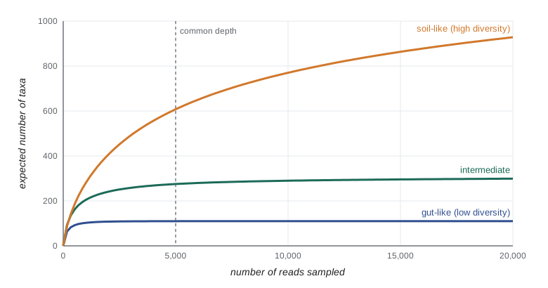

The simulated sample detects most but not all of the 400 taxa, and the rarefaction curve is still creeping upwards at 20,000 reads; Chao1 estimates the total more closely than the raw count. Because richness depends on depth, comparing raw richness between samples sequenced to different depths is misleading. Analysts either rarefy all samples to the same depth, which throws away data, or use statistical methods that model sampling explicitly. Compositional data analysis, such as working with log-ratios of abundances, avoids some of the artifacts of relative abundance.

Beyond 16S: metagenomics and other omics

Shotgun metagenomics sequences all the DNA in a sample rather than one gene. It identifies organisms across all domains, including viruses and fungi, at higher taxonomic resolution, and it reveals the genes present, so it can describe a community’s metabolic potential, its resistance genes (the resistome) and its virulence factors. Assembling reads into contigs and binning them by sequence composition and coverage yields metagenome-assembled genomes (MAGs), near-complete genomes of uncultured organisms. Tens of thousands of MAGs have been reconstructed from environmental and human samples, adding whole new phyla to the tree of life, including the Candidate Phyla Radiation of tiny bacteria with reduced genomes, and the Asgard archaea mentioned in lesson 7. Metatranscriptomics (RNA), metaproteomics (proteins) and metabolomics show which genes are active and which compounds are produced, and stable-isotope probing, in which a labeled substrate is fed to a community and the labeled DNA or cells are then identified, links particular organisms to particular processes.

The human microbiome

The human body carries microbial communities on the skin and in the mouth, airways, urogenital tract and above all the large intestine. The colon contains around 4 × 10¹³ bacterial cells, similar to the number of human cells in the body (the oft-quoted ratio of 10 microbial cells to every human cell was revised in 2016 to about 1.3 to 1), together with archaea, fungi, protists and a vast number of phages. The gut microbiota is dominated by two phyla, Bacillota (formerly Firmicutes) and Bacteroidota, and includes hundreds of species per person, with large differences between individuals. The Human Microbiome Project, launched by the US National Institutes of Health in 2007, and the Canadian Microbiome Initiative of the Canadian Institutes of Health Research, among other projects, cataloged these communities in healthy people.

Colonization begins at birth. Infants born vaginally acquire bacteria resembling their mothers’ vaginal and gut microbiota, whereas those born by cesarean section are first colonized by skin and hospital organisms, though the differences mostly fade within months. Breast milk contains oligosaccharides that infants cannot digest but that feed Bifidobacterium species. The community becomes adult-like by about age three and is then shaped by diet, medications, geography and age. Gut microbes ferment dietary fiber into short-chain fatty acids that nourish the colon lining (lesson 6), synthesize vitamins such as K and some B vitamins, transform bile acids and drugs, train the developing immune system and protect against pathogens by occupying niches and producing inhibitory compounds, a property called colonization resistance.

Antibiotics disrupt colonization resistance, and the most dramatic consequence is infection with Clostridioides difficile, which can cause severe and recurrent diarrhea. For patients with repeated recurrences, fecal microbiota transplantation (FMT), the transfer of stool from a screened healthy donor, cures about 80 to 90 percent of cases in trials, far better than repeated antibiotic courses. It is the clearest evidence that restoring a microbial community can treat disease. FMT carries risks, including transmission of resistant organisms from inadequately screened donors, and regulators treat it as a biological drug; standardized microbiome products derived from donor stool have been approved for preventing recurrent C. difficile infection in the United States since 2022 and 2023.

Beyond C. difficile, associations have been reported between gut microbiome composition and conditions ranging from inflammatory bowel disease and obesity to diabetes, allergy, depression and responses to cancer immunotherapy. Most of these findings are correlations, and many are not consistent between studies. Causation runs in both directions: disease, diet and medication change the microbiome as much as the microbiome changes health. Mouse experiments in which germ-free animals receive human microbiota can test causal hypotheses, but mice are not people. Commercial direct-to-consumer microbiome tests and many probiotic claims go well beyond the evidence. In the United States, most probiotics are sold as dietary supplements under the Dietary Supplement Health and Education Act of 1994, which does not require pre-market proof of efficacy; manufacturers may make structure–function claims but not claims to treat disease. A skeptical reading of microbiome science asks what was measured (relative or absolute abundance, which genes), how large the effect is, whether it replicates, and whether there is evidence from intervention trials rather than associations.