
AI-340 · Lesson 9 of 12 · 28 min
Dense retrieval and retrieval-augmented generation
Language models store a great deal of knowledge in their weights, but that knowledge is frozen at training time, imperfect for rare facts, and absent for private documents such as a company's policies or a hospital's procedures. Retrieval-augmented generation (RAG) addresses this by searching a collection of documents for passages relevant to each question and supplying them to the model in the prompt, so it can answer from current, specific and citable sources. Keyword search with BM25 is implemented in code in Lesson 12; this lesson covers the dense retrieval methods that complement it, how embedding models are trained, how vector indexes search millions of passages quickly, how keyword and dense results are combined and reranked, how documents are chunked, and how RAG systems are built and evaluated.
Sparse and dense retrieval
Sparse retrieval methods such as TF-IDF and BM25 represent documents and queries as vectors over the vocabulary, with nonzero weights only for words that appear. They match exact terms well, which suits names, codes and rare words, and need no training, but they miss documents that express the same meaning in different words: a query about "terminating an employee" may not match a policy about "dismissal". Dense retrieval represents each query and passage as a vector of a few hundred to a few thousand dimensions produced by a neural encoder, and scores relevance by the dot product or cosine similarity:
Because similar meanings map to nearby vectors, dense retrieval handles paraphrases and synonyms, and multilingual encoders can match a French query with an English passage. Its weaknesses are the mirror image: it can miss exact identifiers and rare terms, needs training data from a similar domain to work well, and its errors are harder to explain.
| Aspect | Sparse (BM25) | Dense (embeddings) |
|---|---|---|
| Representation | weighted terms, mostly zeros | dense vectors of 384 to 4,096 numbers |
| Strengths | exact terms, names, codes, rare words; no training | paraphrases, synonyms, cross-lingual matching |
| Weaknesses | vocabulary mismatch | exact identifiers, out-of-domain text |
| Index | inverted index of terms | vector index (approximate nearest neighbor) |
| Explainability | matched terms are visible | similarity is opaque |
Dual encoders and their training
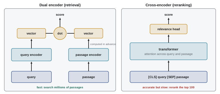
The standard dense retriever is a dual encoder (also called a bi-encoder): one transformer encoder maps the query to a vector, another (often with shared weights) maps each passage, and passages are encoded once, ahead of time, and stored in an index. At query time only the query must be encoded, so search over millions of passages takes milliseconds. Encoders are typically BERT-like models (Lesson 7) whose output vectors are pooled, by taking the [CLS] vector or averaging token vectors, and normalized.
Dual encoders are trained with contrastive learning on pairs of queries and relevant passages, from sources such as search logs, question-answer sites, titles paired with articles, or synthetic questions generated by a language model for each passage. The InfoNCE loss treats retrieval as classification: for a query \(q\) with relevant passage \(p^+\) and negatives \(p_1^-, \ldots, p_n^-\),
where the temperature \(\tau\) controls how sharply the loss focuses on the hardest negatives. An efficient trick is in-batch negatives: in a batch of \(B\) query-passage pairs, each query uses the other \(B - 1\) passages as negatives, so large batches give many negatives at no extra encoding cost.
import numpy as np

# InfoNCE loss with in-batch negatives for a dual-encoder retriever.
# Row i of Q is a query embedding; row i of P is its relevant passage. Other passages in the batch act as negatives.
rng = np.random.default_rng(0)
B, d = 32, 64

def normalize(X):
    return X / np.linalg.norm(X, axis=1, keepdims=True)

def info_nce(Q, P, tau):
    S = Q @ P.T / tau                                   # similarity of every query to every passage
    S = S - S.max(axis=1, keepdims=True)
    log_p = S - np.log(np.exp(S).sum(axis=1, keepdims=True))
    return -np.mean(np.diag(log_p)), np.mean(S.argmax(axis=1) == np.arange(B))

topic = rng.normal(size=d)                                # passages in a batch share a topic, so negatives are similar
P = normalize(topic + 0.8 * rng.normal(size=(B, d)))
for noise, label in ((8.0, "untrained encoder"), (3.0, "partly trained"), (1.0, "well trained")):
    Q = normalize(P + noise * rng.normal(size=(B, d)) / np.sqrt(d))
    for tau in (0.05, 0.5):
        loss, acc = info_nce(Q, P, tau)
        print(f"{label:18s} cos(q, p+) = {np.mean(np.sum(Q * P, axis=1)):.2f}, temperature {tau}: loss {loss:.3f}, in-batch top-1 {acc:.2f}")
print(f"loss of random guessing among {B} passages: ln {B} = {np.log(B):.3f}")untrained encoder cos(q, p+) = 0.15, temperature 0.05: loss 3.147, in-batch top-1 0.16 untrained encoder cos(q, p+) = 0.15, temperature 0.5: loss 3.312, in-batch top-1 0.16 partly trained cos(q, p+) = 0.28, temperature 0.05: loss 2.235, in-batch top-1 0.31 partly trained cos(q, p+) = 0.28, temperature 0.5: loss 3.220, in-batch top-1 0.31 well trained cos(q, p+) = 0.71, temperature 0.05: loss 0.222, in-batch top-1 0.97 well trained cos(q, p+) = 0.71, temperature 0.5: loss 2.852, in-batch top-1 0.97 loss of random guessing among 32 passages: ln 32 = 3.466
An untrained encoder ranks the correct passage first among 32 only 16% of the time, not far above the 3% of random guessing, because the passages share a topic, and its loss is near \(\ln 32\). As training brings query and passage vectors together, the loss falls and top-1 accuracy rises to 97%. At the higher temperature the loss stays high even for a good encoder because its probabilities are spread out, so the gradient pushing hard negatives away is weak; small temperatures around 0.01 to 0.05 are typical. Training is much more effective with hard negatives, passages that look relevant but are not, mined with BM25 or an earlier version of the retriever, because random negatives are too easy to teach fine distinctions.
Embedding models in practice
General-purpose text embedding models, trained on large and varied collections of pairs and compared on public benchmarks such as MTEB, are the usual starting point. Choices include the embedding dimension (larger is often more accurate but costs storage and search time), the maximum input length, multilingual coverage, and whether the model expects instructions or prefixes such as "query:" and "passage:". Some models are trained so that vectors can be truncated to fewer dimensions with modest loss of accuracy. For specialized domains such as law, medicine or engineering standards, fine-tuning an embedding model on in-domain pairs, possibly synthetic, often gives large gains. Embeddings from different models are not comparable, so changing the model means re-encoding the whole collection.
Late interaction
A single vector per passage compresses away detail. Late-interaction models such as ColBERT keep one vector per token and score a query against a passage by summing, for each query token, its maximum similarity to any passage token. They match fine-grained terms better than single-vector models while still allowing passages to be encoded in advance, at the cost of much larger indexes.
Approximate nearest-neighbor search
Finding the exact top-k vectors means comparing the query with every vector, which is too slow for collections of tens of millions. Approximate nearest-neighbor (ANN) indexes trade a little recall for large speed-ups:
- Inverted file (IVF) indexes cluster the vectors with k-means into lists and, at query time, search only the nprobe lists whose centroids are nearest to the query.
- Graph indexes such as HNSW connect each vector to its near neighbors in a layered graph and search by walking greedily toward the query; they give excellent recall and speed and are the default in many vector databases.
- Product quantization (PQ) compresses vectors by splitting them into subvectors and replacing each with the index of the nearest of 256 codebook entries, reducing memory by 10 to 50 times, often combined with IVF.
import numpy as np

# Approximate nearest-neighbour search with an inverted file (IVF) index:
# cluster the vectors, then search only the nprobe clusters nearest to the query.
rng = np.random.default_rng(0)
n, d, k = 20000, 32, 10
centres = rng.normal(size=(50, d))
X = centres[rng.integers(0, 50, n)] + 1.2 * rng.normal(size=(n, d))
X = X / np.linalg.norm(X, axis=1, keepdims=True)
queries = X[rng.choice(n, 200, replace=False)] + 0.1 * rng.normal(size=(200, d))

# k-means with 100 lists
nlist = 100
C = X[rng.choice(n, nlist, replace=False)]
for _ in range(15):
    assign = np.argmax(X @ C.T, axis=1)
    C = np.array([X[assign == j].mean(axis=0) if np.any(assign == j) else C[j] for j in range(nlist)])
    C = C / np.linalg.norm(C, axis=1, keepdims=True)
assign = np.argmax(X @ C.T, axis=1)

exact = np.argsort(-(queries @ X.T), axis=1)[:, :k]
for nprobe in (1, 4, 16, 100):
    recall, scanned = 0.0, 0
    for qi, q in enumerate(queries):
        lists = np.argsort(-(C @ q))[:nprobe]
        cand = np.where(np.isin(assign, lists))[0]
        top = cand[np.argsort(-(X[cand] @ q))[:k]]
        recall += len(set(top) & set(exact[qi])) / k
        scanned += len(cand)
print(f"nprobe {nprobe:3d}: recall@{k} {recall / len(queries):.3f}, vectors scanned per query {scanned / len(queries):7.0f} of {n}")nprobe 1: recall@10 0.581, vectors scanned per query 242 of 20000 nprobe 4: recall@10 0.876, vectors scanned per query 820 of 20000 nprobe 16: recall@10 0.977, vectors scanned per query 3194 of 20000 nprobe 100: recall@10 1.000, vectors scanned per query 20000 of 20000
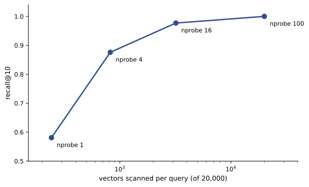
Probing more lists raises recall at the cost of more computation. The right setting depends on the application: a RAG system that passes the top 10 passages to a reranker can tolerate slightly lower recall than one that shows results directly. Index parameters should be tuned by measuring recall against exact search on a sample of real queries.
Hybrid search and reranking
Because sparse and dense retrieval fail on different queries, combining them usually beats either alone. A simple, robust method is reciprocal rank fusion (RRF), which ignores the incomparable raw scores and combines ranks:
with \(k\) typically 60. A document ranked highly by both methods rises to the top, and a document found by only one still appears.
Worked problem
Reciprocal rank fusion
BM25 ranks passages A, B, C first, second and third; dense retrieval ranks C, D, A. Using \(k = 60\), compute the fused order.
Show solution
- A: \(1/61 + 1/63 = 0.01639 + 0.01587 = 0.03226\).
- C: \(1/63 + 1/61 = 0.03226\), the same as A.
- B: \(1/62 = 0.01613\). D: \(1/62 = 0.01613\).
Answer: A and C tie at the top because each was found by both methods; B and D, each found by only one, follow. Ties are broken by a further rule, such as a reranker score.
Retrieval quality is then improved with a reranker, usually a cross-encoder: a transformer that reads the query and a candidate passage together and outputs a relevance score. Because it attends across query and passage, it is far more accurate than a dual encoder, but too slow to apply to the whole collection, so it rescores only the top 20 to 100 candidates. Language models can also serve as rerankers. A typical pipeline therefore has stages: fast, high-recall retrieval (hybrid), then slower, high-precision reranking, then generation.
Chunking and indexing documents
Documents are split into chunks small enough to embed precisely and to fit several in a prompt, but large enough to carry their meaning. Good chunking is often the difference between a RAG system that works and one that does not:
- Split on structure where possible: headings, sections, paragraphs, table rows or code functions, rather than at a fixed character count.
- Typical chunk sizes are 200 to 800 tokens, with a small overlap so sentences at boundaries are not lost.
- Add context to each chunk: the document title, section heading and date, so that a chunk saying "the limit is 30 days" carries what the limit applies to.
- Handle tables, figures and scanned pages carefully, with layout-aware parsing or descriptions generated by a vision model.
- Store metadata such as source, date, access permissions and language for filtering at query time, and enforce permissions so that users only retrieve documents they are allowed to see.
- Keep the index up to date as documents change, and remove superseded versions.
Generation with retrieved context
The retrieved passages are placed in the prompt with the question and instructions such as: answer using only the passages below; cite the passage number for each claim; if the passages do not contain the answer, say so. Practical refinements include:
- Query rewriting: turn a conversational follow-up ("what about for contractors?") into a standalone query, or generate several query variants.
- Ordering: models attend best to information at the start and end of long contexts, so place the most relevant passages there.
- Iterative or agentic retrieval: let the model issue further searches when the first results are insufficient (Lesson 11).
- Long-context models can take entire documents, which reduces the need for chunking in small collections, but retrieval remains cheaper, faster and more focused for large ones.
Evaluating RAG systems
A RAG system can fail at retrieval (the right passage was not found), at generation (the passage was found but the answer ignored or misread it), or both, so the stages are evaluated separately and together:
- Retrieval: recall@k (did the relevant passage appear in the top k?), mean reciprocal rank, and nDCG on a labeled set of questions and relevant passages.
- Faithfulness or groundedness: is every claim in the answer supported by the retrieved passages?
- Answer relevance and correctness: does the answer address the question and match a reference answer?
- Citation accuracy: do cited passages actually support the claims attached to them?
- Abstention: does the system decline when the collection does not contain the answer?
Language models are often used as judges to score faithfulness and correctness at scale, but their judgments should be checked against human ratings on a sample (Lesson 12). A good evaluation set includes real user questions, questions requiring several passages, questions whose answers are not in the collection, and questions about recently changed documents.
Common mistakes
MistakeUsing dense retrieval alone for queries full of codes and names.
InsteadUse hybrid search with BM25 for exact terms.
MistakeChunking at fixed character counts that split tables and sentences.
InsteadChunk on document structure and add titles and headings to chunks.
MistakeIgnoring access permissions in the index.
InsteadStore permissions as metadata and filter every query.
MistakeEvaluating only the final answers.
InsteadMeasure retrieval recall and faithfulness separately to locate failures.
MistakeTraining a retriever with random negatives only.
InsteadMine hard negatives that look relevant but are not.
Summary and key terms
- RAG grounds a language model in retrieved passages, giving current, specific and citable answers.
- Dense retrieval matches meaning with embeddings; sparse retrieval matches exact terms; hybrid search combines them.
- Dual encoders are trained contrastively with InfoNCE, in-batch negatives and hard negatives.
- ANN indexes such as IVF, HNSW and PQ trade a little recall for large speed and memory savings.
- Cross-encoder rerankers rescore the top candidates for precision.
- Chunking, metadata, permissions and evaluation of both retrieval and faithfulness determine RAG quality.
- Dense retrieval
- Retrieval by similarity of learned embedding vectors.
- Dual encoder
- Separate encoding of queries and passages into vectors.
- InfoNCE
- A contrastive loss treating retrieval of the positive among negatives as classification.
- Hard negative
- A passage that appears relevant but is not.
- ANN search
- Approximate nearest-neighbor search trading recall for speed.
- HNSW
- A layered graph index for approximate nearest-neighbor search.
- Reciprocal rank fusion
- Combining rankings by summing 1/(k + rank).
- Cross-encoder
- A model scoring a query and passage read together.
- Chunking
- Splitting documents into passages for indexing.
- Faithfulness
- Support of an answer's claims by the retrieved sources.
Practice problems
Work each problem on paper first, then reveal the answer to check.
Give one strength of BM25 over dense retrieval.
Show answer
Exact matching of names, codes and rare terms.
Why are passages encoded ahead of time in a dual encoder?
Show answer
So only the query must be encoded at search time.
How many in-batch negatives does each query have in a batch of 64?
Show answer
63.
What InfoNCE loss corresponds to random guessing among 16 passages?
Show answer
\(\ln 16 \approx 2.77\).
What does nprobe control in an IVF index?
Show answer
How many clusters are searched, trading speed for recall.
RRF score for a document ranked 1st and 5th with k = 60?
Show answer
\(1/61 + 1/65 \approx 0.0318\).
Why not apply a cross-encoder to the whole collection?
Show answer
It is too slow; each passage must be processed with the query.
What context should be added to chunks?
Show answer
Document title, section heading, date.
What is faithfulness?
Show answer
Whether the answer's claims are supported by retrieved passages.
Name a question type to include in a RAG evaluation set.
Show answer
Questions whose answers are not in the collection, multi-passage questions, real user questions.
Lesson quiz · 5 questions
Score 60% or more to complete this lesson.
Create a free account to save your progress, take quizzes and earn a certificate.