Attention and the transformer

In 2017, a team at Google published "Attention Is All You Need", introducing the transformer: an architecture for sequences that uses no recurrence at all, relying entirely on attention to let every token gather information from every other token. Transformers trained faster than RNNs because all positions are processed in parallel, captured long-range dependencies directly, and scaled remarkably well with more data and computation. Within a few years they had replaced RNNs across NLP and spread to vision, speech, protein structure and more. Every large language model in use today is a transformer or a close variant. This lesson builds the transformer from its parts: scaled dot-product attention, multiple heads, positional information, the transformer block, and the encoder, decoder and encoder-decoder families, ending with the costs that govern how these models are trained and served.

Attention as soft lookup

Attention can be understood as a soft dictionary lookup. Each position produces a query (what it is looking for), a key (what it offers to be matched against) and a value (the information it passes on). The query of one position is compared with the keys of all positions; the comparison scores are turned into weights with a softmax; and the output is the weighted average of the values. Unlike a real dictionary, which returns exactly one entry, attention returns a blend weighted by relevance, and because everything is differentiable, the model learns what to look for and what to offer.

For a sequence of \(n\) token vectors stacked as rows of \(X\), learned matrices project them into queries, keys and values: \(Q = XW_Q\), \(K = XW_K\), \(V = XW_V\). Scaled dot-product attention is then:

The \(n \times n\) matrix \(QK^\top\) holds the score of every query against every key. Each row of the softmax output is a probability distribution saying how much each position attends to every other, and multiplying by \(V\) mixes the value vectors accordingly. Because the queries, keys and values all come from the same sequence, this is called self-attention.

import numpy as np

rng = np.random.default_rng(0)
tokens = ["the", "cat", "sat", "on", "it"]
n, d_model, d_k = len(tokens), 16, 8
X = rng.normal(0, 1, (n, d_model))              # token embeddings (random for illustration)
Wq, Wk, Wv = (rng.normal(0, d_model ** -0.5, (d_model, d_k)) for _ in range(3))

def softmax(z):
    z = z - z.max(axis=-1, keepdims=True)
    e = np.exp(z)
    return e / e.sum(axis=-1, keepdims=True)

def attention(X, causal):
    Q, K, V = X @ Wq, X @ Wk, X @ Wv
    scores = Q @ K.T / np.sqrt(d_k)
    if causal:                                    # each position sees only itself and earlier ones
        scores = np.where(np.tril(np.ones((n, n))) == 1, scores, -np.inf)
    A = softmax(scores)
    return A, A @ V

np.set_printoptions(precision=2, suppress=True)
A, out = attention(X, causal=True)
print("causal attention weights (rows = query position):")
print(A)
print("rows sum to", A.sum(axis=1))
print("output shape:", out.shape)
# changing a later token cannot affect earlier outputs under the causal mask
X2 = X.copy(); X2[4] += 5
_, out2 = attention(X2, causal=True)
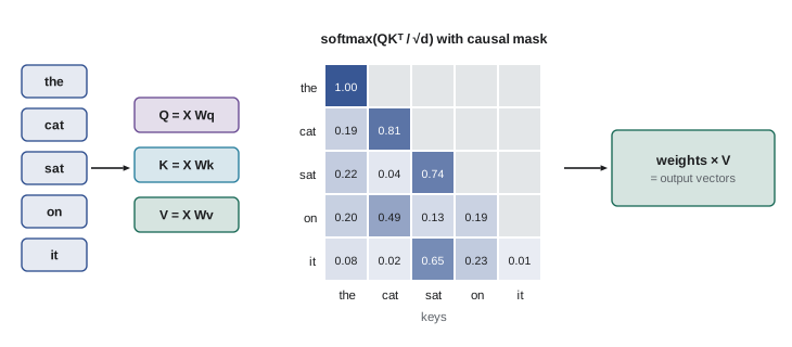
print("max change in outputs 0-3:", float(abs(out2[:4] - out[:4]).max()), "  output 4:", round(float(abs(out2[4] - out[4]).max()), 2))

causal attention weights (rows = query position):
[[1.   0.   0.   0.   0.  ]
 [0.19 0.81 0.   0.   0.  ]
 [0.22 0.04 0.74 0.   0.  ]
 [0.2  0.49 0.13 0.19 0.  ]
 [0.08 0.02 0.65 0.23 0.01]]
rows sum to [1. 1. 1. 1. 1.]
output shape: (5, 8)
max change in outputs 0-3: 0.0   output 4: 6.83

In a language model, a token must not see the tokens it is trying to predict, so a causal mask sets the scores for future positions to \(-\infty\) before the softmax, giving them weight zero. The weight matrix is lower triangular: the first token can attend only to itself, and the last to everything. The check at the end confirms the masking works: changing the last token leaves the outputs at positions 0 to 3 exactly unchanged. Because the mask enforces causality, a model can be trained on all positions of a sequence in parallel, each predicting its next token, while still being usable for left-to-right generation.

Why scale by the square root of d

If the components of queries and keys are independent with mean 0 and variance 1, their dot product over \(d_k\) dimensions has variance \(d_k\), so its standard deviation grows as \(\sqrt{d_k}\). Large scores push the softmax into saturation, where almost all the weight goes to one position and gradients become tiny. Dividing by \(\sqrt{d_k}\) restores unit variance regardless of dimension.

import numpy as np

rng = np.random.default_rng(0)
def softmax(z):
    e = np.exp(z - z.max(axis=-1, keepdims=True))
    return e / e.sum(axis=-1, keepdims=True)

n = 64
print(" d_k   score std (raw)  max weight raw   max weight scaled")
for d in (16, 64, 256, 1024):
    q = rng.normal(0, 1, (200, d)); k = rng.normal(0, 1, (n, d))
    raw = q @ k.T
    a_raw = softmax(raw).max(axis=1).mean()
    a_scaled = softmax(raw / np.sqrt(d)).max(axis=1).mean()
    print(f"{d:5d}   {raw.std():10.1f}      {a_raw:10.3f}       {a_scaled:10.3f}")

 d_k   score std (raw)  max weight raw   max weight scaled
   16          3.9           0.571            0.103
   64          8.0           0.776            0.105
  256         16.1           0.877            0.106
 1024         32.2           0.949            0.109

Without scaling, the average largest weight among 64 keys rises from 0.57 at \(d_k = 16\) to 0.95 at \(d_k = 1024\): attention collapses onto one position and learning slows. With scaling it stays near 0.1 at every dimension, so attention can spread across several positions and gradients flow.

Multi-head attention

A single attention operation produces one weighted average per position, so it can follow only one kind of relationship at a time. Multi-head attention runs \(h\) attention operations in parallel, each with its own smaller projections of dimension \(d_k = d_{model}/h\), then concatenates their outputs and applies an output projection \(W_O\):

Different heads learn different patterns: studies of trained models have found heads that attend to the previous token, heads that link a pronoun to its antecedent, heads that track syntactic relations such as verbs and their objects, and "induction heads" that find an earlier occurrence of the current token and copy what followed it, a mechanism behind in-context learning. Because each head has dimension \(d_{model}/h\), multi-head attention costs about the same as a single full-width head.

Position information

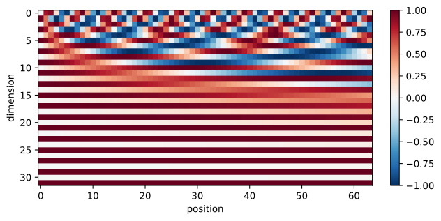
Attention treats its input as a set: permuting the tokens permutes the outputs in the same way, so "dog bites man" and "man bites dog" would look alike. Transformers therefore add information about position. The original transformer added fixed sinusoidal positional encodings to the token embeddings, with each pair of dimensions oscillating at a different frequency:

BERT and GPT-2 instead learned a separate embedding for each position, which limits them to the maximum length seen in training. Most current large language models use rotary position embeddings (RoPE), which rotate each pair of query and key dimensions by an angle proportional to the position. Because rotating both vectors changes their dot product only through the difference of their angles, attention scores depend only on the relative offset between tokens, not their absolute positions.

import numpy as np

d = 16
freqs = 1.0 / 10000 ** (np.arange(0, d, 2) / d)     # one frequency per pair of dimensions

def sinusoidal(pos):
    pe = np.zeros(d)
    pe[0::2] = np.sin(pos * freqs); pe[1::2] = np.cos(pos * freqs)
    return pe

print("sinusoidal: PE(p) . PE(p + 3) for p = 0, 10, 50:",
      [round(float(sinusoidal(p) @ sinusoidal(p + 3)), 4) for p in (0, 10, 50)])

def rope(x, pos):                                   # rotate each pair of dimensions by pos * freq
    x1, x2 = x[0::2], x[1::2]
    c, s = np.cos(pos * freqs), np.sin(pos * freqs)
    out = np.empty_like(x)
    out[0::2] = x1 * c - x2 * s; out[1::2] = x1 * s + x2 * c
    return out

rng = np.random.default_rng(0)
q, k = rng.normal(size=d), rng.normal(size=d)
for m, n in ((5, 2), (105, 102), (1005, 1002), (5, 4)):
    print(f"RoPE: query at {m:4d}, key at {n:4d} (offset {m - n}): score = {rope(q, m) @ rope(k, n):.4f}")
print("norm preserved:", round(float(np.linalg.norm(rope(q, 77))), 4), "=", round(float(np.linalg.norm(q)), 4))

sinusoidal: PE(p) . PE(p + 3) for p = 0, 10, 50: [5.5431, 5.5431, 5.5431]
RoPE: query at    5, key at    2 (offset 3): score = 2.7754
RoPE: query at  105, key at  102 (offset 3): score = 2.7754
RoPE: query at 1005, key at 1002 (offset 3): score = 2.7754
RoPE: query at    5, key at    4 (offset 1): score = 2.5418
norm preserved: 3.674 = 3.674

The dot product of sinusoidal encodings three positions apart is the same (5.5431) at every position, and the RoPE score for a query and key three positions apart is identical at positions 5, 105 and 1005, changing only when the offset changes. Rotation also preserves vector length. Relative position methods like RoPE, often with adjustments to the rotation frequencies, help models extend to contexts longer than those seen in training.

The transformer block

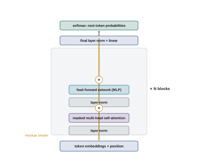
A transformer is a stack of identical blocks. Each block has two sublayers, each wrapped in a residual connection and layer normalization:

• Multi-head self-attention, which moves information between positions.
• A position-wise feed-forward network (MLP), applied to each position independently, which transforms the information at each position. It typically expands the dimension by a factor of about 4 (for example from 768 to 3072) with a nonlinearity such as GELU, then projects back. Many modern models use a gated variant (SwiGLU) with three matrices.

The residual connections let each block add a refinement to a running "residual stream" rather than replacing it, which keeps gradients flowing through dozens of layers, much as the LSTM cell state did through time. The original transformer applied layer normalization after each residual addition (post-norm); most current models apply it before each sublayer (pre-norm, as above), which trains more stably in deep networks. A final layer normalization and a linear layer, often sharing weights with the input embedding, produce logits over the vocabulary.

Encoders, decoders and both

Transformers come in three families:

• Encoder-only models (BERT, RoBERTa) use bidirectional self-attention with no causal mask, so every token sees the whole input. They are pretrained by masked language modeling: about 15% of tokens are hidden and the model predicts them from both sides. Encoders produce rich contextual representations and excel at classification, tagging, retrieval and sentence embeddings, but do not generate text naturally.
• Decoder-only models (the GPT family and most modern large language models) use causal self-attention and are pretrained to predict the next token. They generate text and, at sufficient scale, perform many tasks from instructions and examples in the prompt.
• Encoder-decoder models (the original transformer, T5, BART) encode an input bidirectionally and decode an output causally, with cross-attention layers in which decoder queries attend to encoder keys and values. They suit translation and summarization, where input and output are distinct.

Since about 2020 the decoder-only design has dominated because a single next-token objective on huge amounts of text, followed by fine-tuning, yields one model that can do almost every task (AI-410). Encoder models remain widely used where efficiency matters, for example in search, classification and embedding services.

Costs: parameters, computation and memory

The cost of a transformer is dominated by its matrix multiplications. Each block has about \(4d^2\) parameters in attention (Q, K, V and output projections) and \(8d^2\) in a standard MLP with 4x expansion, so about \(12d^2\) per layer. A forward pass costs about 2 floating-point operations per parameter per token (one multiply and one add), and training costs about three times as much (forward plus backward), the basis of the common estimate of \(6ND\) training FLOPs for \(N\) parameters and \(D\) tokens.

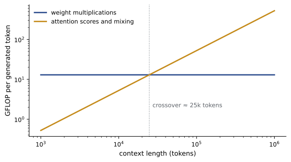
Attention adds a cost that grows with the square of the sequence length \(n\): the score matrix has \(n^2\) entries per head per layer. For short sequences this is small compared with the weight multiplications, but at contexts of hundreds of thousands of tokens it dominates, which has motivated efficient attention algorithms (FlashAttention, which avoids storing the full matrix), sparse and sliding-window attention, and the recurrent alternatives mentioned in Lesson 4.

During generation, a model produces one token at a time. To avoid recomputing the keys and values of all earlier tokens at every step, it stores them in a key-value (KV) cache, whose size grows with the context length, the number of layers and the number of key-value heads. Grouped-query attention (GQA) shares each key-value head among several query heads, shrinking the cache several-fold with little loss of quality.

def count(name, d, layers, ff, vocab, heads, kv_heads, gated, tied, ctx):
    attn = d * d * 2 + 2 * d * (d // heads) * kv_heads      # Q and output, plus K and V
    mlp = (3 if gated else 2) * d * ff
    per_layer = attn + mlp
    emb = vocab * d * (1 if tied else 2)                 # input embedding, plus output layer if untied
    total = layers * per_layer + emb
    flops_per_token = 2 * (total - emb)                    # one multiply-add per weight
    kv_bytes = 2 * layers * (d // heads) * kv_heads * 2    # K and V, 16-bit numbers
    print(f"{name}: {total / 1e9:.2f} B parameters ({layers * per_layer / 1e9:.2f} B in layers,"
          f" {emb / 1e9:.2f} B embeddings)")
    print(f"   forward FLOPs per token ~ {flops_per_token / 1e9:.1f} GFLOP;"
          f" KV cache {kv_bytes / 1024:.0f} KiB per token, {kv_bytes * ctx / 2**30:.2f} GiB for {ctx} tokens")

count("GPT-2 small", 768, 12, 3072, 50257, 12, 12, False, True, 1024)
count("7B decoder (multi-head)", 4096, 32, 11008, 32000, 32, 32, True, False, 4096)
count("8B decoder (grouped-query, 8 KV heads)", 4096, 32, 14336, 128256, 32, 8, True, False, 8192)

GPT-2 small: 0.12 B parameters (0.08 B in layers, 0.04 B embeddings)
   forward FLOPs per token ~ 0.2 GFLOP; KV cache 36 KiB per token, 0.04 GiB for 1024 tokens
7B decoder (multi-head): 6.74 B parameters (6.48 B in layers, 0.26 B embeddings)
   forward FLOPs per token ~ 13.0 GFLOP; KV cache 512 KiB per token, 2.00 GiB for 4096 tokens
8B decoder (grouped-query, 8 KV heads): 8.03 B parameters (6.98 B in layers, 1.05 B embeddings)
   forward FLOPs per token ~ 14.0 GFLOP; KV cache 128 KiB per token, 1.00 GiB for 8192 tokens

The counts match the published sizes of these architectures: about 124 million parameters for GPT-2 small (the output layer shares the input embedding), 6.7 billion for a 7B model with multi-head attention, and 8.0 billion for an 8B model with grouped-query attention and a 128,000-token vocabulary. Each generated token costs about 13 to 14 GFLOP for the 7B and 8B models. Grouped-query attention with 8 key-value heads cuts the KV cache from 512 KiB to 128 KiB per token, so the 8B model's cache for an 8192-token context (1 GiB) is half that of the 7B model for 4096 tokens. For a server handling many conversations at once, the KV cache, not the weights, often limits how many users fit on a GPU.

Lesson 7 shows how transformers are pretrained on vast amounts of text, and Lesson 10 how they are made efficient to run.