
AI-340 · Lesson 10 of 12 · 28 min
Efficient NLP: adaptation, compression and fast inference
Large language models are expensive to adapt and to run. Fully fine-tuning a 7-billion-parameter model needs over 100 GB of accelerator memory, serving it to many users needs fleets of GPUs, and every generated token passes through all of its layers. For most organizations, the practical questions are therefore about efficiency: how to adapt a large model to a task with modest hardware, how to make it smaller and faster without losing much accuracy, and how to serve it at low cost and latency. This lesson covers parameter-efficient fine-tuning with LoRA, quantization, knowledge distillation and pruning, the key-value cache and memory management, and decoding accelerations such as speculative decoding, ending with how to choose a model size for an application.
Why efficiency matters
Costs arise at two stages. Adaptation (fine-tuning) is a one-time or periodic cost dominated by memory: weights, gradients and optimizer states must all fit on accelerators. Inference is a recurring cost that grows with the number of users and the length of their requests, and over the life of a deployed model it usually exceeds the training cost. Inference has two phases with different bottlenecks: processing the prompt (prefill) is compute-bound and parallel over tokens, while generating the output (decode) produces one token at a time and is limited by the speed of reading the weights and cache from memory. Efficiency also matters for privacy and access: a model small enough to run on a laptop or phone keeps data on the device and works offline.
Parameter-efficient fine-tuning
Full fine-tuning updates every weight and stores a full copy of the model per task. Parameter-efficient fine-tuning (PEFT) freezes the pretrained weights and trains a small number of new parameters. Approaches include adapters (small bottleneck layers inserted in each transformer block), prefix and prompt tuning (trainable vectors prepended to the input or to each layer's keys and values), and, most widely used, low-rank adaptation.
LoRA
Low-rank adaptation (LoRA) is based on the observation that the weight changes needed to adapt a model to a task have low intrinsic rank. For a frozen weight matrix \(W_0\) of size \(d \times k\), LoRA learns the update as the product of two thin matrices:
Only \(A\) and \(B\) are trained, \(r(d + k)\) parameters instead of \(dk\). \(B\) is initialized to zero so training starts from the pretrained model, and \(\alpha\) scales the update. After training, \(BA\) can be added to \(W_0\), so inference has no extra cost, or several LoRA adapters can be kept and swapped in for different tasks or customers while sharing one base model in memory.
import numpy as np

# LoRA: replace the update of a d x k weight matrix by a low-rank product B A with rank r.
d = k = 4096
layers, mats = 32, 4                                    # 32 layers, LoRA on the q, k, v and output projections
full = layers * mats * d * k
for r in (4, 16, 64):
    lora = layers * mats * r * (d + k)
    print(f"rank {r:2d}: {lora / 1e6:6.1f} M trainable parameters ({lora / full:.2%} of the {full / 1e6:.0f} M in these matrices)")

# How well can a low-rank update approximate a weight change that is approximately low rank?
rng = np.random.default_rng(0)
n = 512
U = rng.normal(size=(n, 8)); V = rng.normal(size=(8, n))
delta = U @ V / 8 + 0.05 * rng.normal(size=(n, n))       # true change: rank 8 plus small noise
u, s, vt = np.linalg.svd(delta)
for r in (1, 4, 8, 32):
    approx = (u[:, :r] * s[:r]) @ vt[:r]
    err = np.linalg.norm(delta - approx) / np.linalg.norm(delta)
    print(f"best rank-{r:2d} approximation: relative error {err:.3f}")

# Memory for full fine-tuning versus LoRA on a 7B model with Adam, 16-bit weights
P = 7e9
full_gb = P * (2 + 2 + 4 * 3) / 1e9                     # weights, gradients, fp32 master copy and two Adam moments
lora_P = 32 * 4 * 16 * (4096 + 4096)
lora_gb = (P * 2 + lora_P * 16) / 1e9
print(f"full fine-tuning: about {full_gb:.0f} GB before activations; LoRA rank 16: about {lora_gb:.1f} GB")rank 4: 4.2 M trainable parameters (0.20% of the 2147 M in these matrices) rank 16: 16.8 M trainable parameters (0.78% of the 2147 M in these matrices) rank 64: 67.1 M trainable parameters (3.12% of the 2147 M in these matrices) best rank- 1 approximation: relative error 0.917 best rank- 4 approximation: relative error 0.649 best rank- 8 approximation: relative error 0.137 best rank-32 approximation: relative error 0.126 full fine-tuning: about 112 GB before activations; LoRA rank 16: about 14.3 GB
Rank 16 on the attention projections trains under 1% of their parameters. The approximation experiment shows why low rank suffices when the true change is close to low rank: a rank-8 approximation captures almost all of a rank-8 change, and higher ranks add little. Memory falls from over 100 GB for full fine-tuning with Adam to about 14 GB, because gradients and optimizer states are needed only for the small adapter matrices. QLoRA goes further by storing the frozen base model in 4-bit precision while training LoRA adapters in higher precision, allowing models with tens of billions of parameters to be fine-tuned on a single GPU. LoRA usually matches full fine-tuning on narrow tasks, though it can fall short when a task requires learning much new knowledge.
Worked problem
Planning a LoRA fine-tune
A team wants to adapt a 13B-parameter model (40 layers, \(d = 5{,}120\)) to classify support tickets, using LoRA of rank 8 on the query and value projections only. How many parameters are trained, and roughly how much memory do the frozen 16-bit weights need?
Show solution
- Per matrix: \(8 \times (5{,}120 + 5{,}120) = 81{,}920\) parameters.
- Two matrices per layer, 40 layers: \(80 \times 81{,}920 = 6.55\) million parameters.
- Frozen weights: \(13 \times 10^9 \times 2\) bytes \(= 26\) GB, or about 6.5 GB at 4 bits with QLoRA.
Answer: About 6.6 million trainable parameters, 0.05% of the model. With 4-bit base weights the job fits on a single 24 GB GPU with room for activations; at 16 bits it needs a larger card.
Quantization
Quantization stores weights (and sometimes activations and the cache) with fewer bits: 8-bit or 4-bit integers instead of 16-bit floating-point numbers. A group of weights is mapped to integers by dividing by a scale and rounding, and multiplied back by the scale when used. Fewer bits mean smaller models, and because decoding is limited by memory bandwidth, faster generation.
import numpy as np

# Quantizing weights to fewer bits. Per-tensor versus per-group scaling, with a few outlier weights.
rng = np.random.default_rng(0)
W = rng.normal(0, 0.02, size=(1024, 1024))
W[rng.integers(0, 1024, 20), rng.integers(0, 1024, 20)] = 0.5      # rare large outliers, common in LLM weights
x = rng.normal(size=1024)
y = W @ x

def quantize(w, bits):
    levels = 2 ** (bits - 1) - 1
    scale = np.abs(w).max() / levels
    return np.round(w / scale).clip(-levels, levels) * scale

def per_group(w, bits, g):
    flat = w.reshape(-1, g)
    return np.vstack([quantize(row, bits) for row in flat]).reshape(w.shape)

for bits in (8, 4):
    for name, Wq in (("per-tensor", quantize(W, bits)), ("groups of 128", per_group(W, bits, 128)), ("groups of 32", per_group(W, bits, 32))):
        err = np.linalg.norm(Wq @ x - y) / np.linalg.norm(y)
        print(f"{bits}-bit {name:13s}: relative output error {err:.4f}")

for bits in (16, 8, 4):
    print(f"7B-parameter model at {bits} bits: {7e9 * bits / 8 / 1e9:.1f} GB of weights")
# The key-value cache grows with context length: 2 (K and V) x layers x KV heads x head size x tokens x bytes
layers, kv_heads, head = 32, 8, 128
for tokens in (4096, 32768, 131072):
    gb = 2 * layers * kv_heads * head * tokens * 2 / 1e9
print(f"KV cache for one sequence of {tokens} tokens at 16 bits: {gb:.2f} GB")8-bit per-tensor : relative output error 0.0568 8-bit groups of 128: relative output error 0.0071 8-bit groups of 32 : relative output error 0.0056 4-bit per-tensor : relative output error 0.8853 4-bit groups of 128: relative output error 0.1274 4-bit groups of 32 : relative output error 0.0988 7B-parameter model at 16 bits: 14.0 GB of weights 7B-parameter model at 8 bits: 7.0 GB of weights 7B-parameter model at 4 bits: 3.5 GB of weights KV cache for one sequence of 4096 tokens at 16 bits: 0.54 GB KV cache for one sequence of 32768 tokens at 16 bits: 4.29 GB KV cache for one sequence of 131072 tokens at 16 bits: 17.18 GB
A single scale for a whole matrix fails at 4 bits because a few large outlier weights, common in language models, stretch the range so that ordinary weights round to zero. Per-group scales, one per 32 to 128 weights, confine the damage to the groups containing outliers. Simple rounding at 4 bits still introduces noticeable error, so practical methods do better: GPTQ quantizes weights one column at a time and adjusts the remaining weights to compensate for the error, using a small calibration set; AWQ protects the weights that multiply large activations; and formats such as NF4 place quantization levels to match the normal distribution of weights. With such methods, 8-bit models are nearly lossless and 4-bit models typically lose a little accuracy, more for small models and for demanding tasks such as mathematics. Quantization-aware training, which simulates quantization during training, recovers more accuracy at lower bit widths.
| Precision | Bytes per parameter | 7B model | 70B model | Typical quality |
|---|---|---|---|---|
| FP32 | 4 | 28 GB | 280 GB | training master weights |
| BF16 or FP16 | 2 | 14 GB | 140 GB | standard for inference |
| INT8 or FP8 | 1 | 7 GB | 70 GB | nearly lossless |
| INT4 (GPTQ, AWQ, NF4) | 0.5 | 3.5 GB | 35 GB | small loss; popular for local use |
Distillation and pruning
Knowledge distillation trains a small student model to imitate a large teacher. Rather than learning only from the correct labels, the student matches the teacher's full output distribution, softened by a temperature \(T\), which conveys how the teacher ranks wrong answers:
DistilBERT retained about 97% of BERT's benchmark performance with 40% fewer parameters and 60% faster inference. For generative models, distillation often takes the form of training a small model on large amounts of text generated by a large model, or on the teacher's token probabilities; many capable small open models are produced this way. Pruning removes weights, attention heads or entire layers that contribute little. Unstructured pruning (zeroing individual weights) reduces size but speeds inference only on hardware that exploits sparsity; structured pruning removes whole components and gives real speed-ups, usually followed by further training to recover accuracy.
Serving: the key-value cache
In autoregressive generation, each new token attends to all previous tokens. Recomputing the keys and values of the whole prefix at every step would be wasteful, so they are stored in a key-value (KV) cache and only the new token's keys and values are computed. The cache grows linearly with sequence length and with the number of concurrent sequences, and for long contexts it can exceed the size of the weights: the code above shows a 7B-class model with 8 key-value heads needing about 17 GB of cache for a single 128,000-token sequence. Techniques to manage it include:
- Grouped-query and multi-query attention, which share key and value heads among several query heads, reducing the cache by 4 to 8 times with little loss of quality; most recent models use them.
- Paged attention, used in serving engines such as vLLM, which stores the cache in fixed-size blocks like virtual memory pages, eliminating fragmentation and allowing sequences that share a prompt prefix to share cache blocks.
- Prefix (prompt) caching, which keeps the cache for long shared system prompts or documents so later requests skip their prefill.
- Quantizing the cache to 8 or 4 bits, and sliding-window attention, which keeps only recent tokens for some layers.
Continuous batching processes many users' requests together, adding new requests to the batch as others finish, so the GPU reads each weight once for many tokens. It raises throughput several times over static batching. FlashAttention computes attention in tiles that fit in fast on-chip memory, avoiding storing the full attention matrix and speeding up long sequences.
Faster decoding
Decoding one token at a time leaves the accelerator underused, because reading the weights dominates and the arithmetic for one token is small. Speculative decoding exploits this: a small, fast draft model proposes several tokens, and the large target model checks all of them in one parallel forward pass, accepting the longest prefix consistent with its own distribution and correcting the first rejected token. With the acceptance rule of the original method, the output distribution is exactly that of the target model, so quality is unchanged, while speed-ups of 2 to 3 times are common when the draft model guesses well, as it does for predictable text such as code.
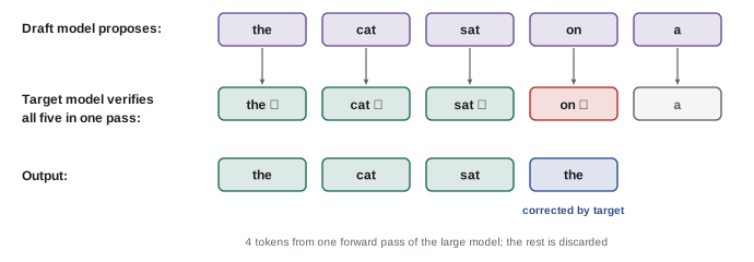
If each draft token is accepted with probability \(a\) independently and the draft proposes \(\gamma\) tokens, the expected number of tokens produced per target pass is
For \(a = 0.8\) and \(\gamma = 4\), this is \((1 - 0.8^5)/0.2 = 3.4\) tokens per pass. Variants dispense with a separate draft model by adding extra prediction heads to the target model (Medusa) or by drafting from n-grams found in the prompt, which works well when outputs copy from the input, as in editing and RAG.
Choosing a model and deployment
Efficient deployment starts with choosing the smallest model that meets the quality bar. A practical process:
- Define the task and build an evaluation set from real examples (Lesson 12).
- Measure a strong large model to establish what is achievable, then test smaller models, with prompting, RAG or fine-tuning.
- Consider a fine-tuned small model for narrow, high-volume tasks such as classification and extraction; it is often as accurate as a general large model at a fraction of the cost.
- Route requests: send easy queries to a small model and hard ones to a large model, using a classifier or the small model's confidence.
- Quantize and use an efficient serving engine; measure latency (time to first token and tokens per second) and cost per request under realistic load.
- Weigh hosted APIs, which need no infrastructure but send data to a provider, against self-hosting open models, which gives control over data and cost at the price of operations work. Data residency requirements in Canadian privacy law, or sector rules, may favor hosting within Canada.
Common mistakes
MistakeFully fine-tuning a large model for a narrow task.
InsteadTry LoRA or QLoRA first; they need a fraction of the memory.
MistakeQuantizing with one scale per tensor.
InsteadUse per-group scales and calibrated methods such as GPTQ or AWQ.
MistakeIgnoring the KV cache when sizing hardware for long contexts.
InsteadBudget cache memory per sequence times concurrent users.
MistakeAssuming a quantized or distilled model matches the original.
InsteadEvaluate it on the task, especially for reasoning and rare cases.
MistakePicking the largest model by default.
InsteadFind the smallest model that meets the quality bar, and route by difficulty.
Summary and key terms
- Inference usually dominates lifetime cost; decoding is limited by memory bandwidth.
- LoRA trains a low-rank update with under 1% of parameters, and QLoRA adds a 4-bit base model.
- Quantization to 8 or 4 bits shrinks and speeds up models; per-group scales and calibrated methods limit error.
- Distillation trains small students on a teacher's outputs; structured pruning removes components.
- The KV cache grows with context and users; grouped-query attention, paged attention and prefix caching manage it.
- Speculative decoding and continuous batching speed up serving without changing outputs.
- PEFT
- Parameter-efficient fine-tuning, training few new parameters with the base frozen.
- LoRA
- Low-rank adaptation, learning a weight update as a product of thin matrices.
- QLoRA
- LoRA training on a 4-bit quantized base model.
- Quantization
- Representing numbers with fewer bits.
- Knowledge distillation
- Training a student model to imitate a teacher model.
- Pruning
- Removing weights or components that contribute little.
- KV cache
- Stored keys and values of previous tokens used during generation.
- Grouped-query attention
- Sharing key and value heads among groups of query heads.
- Continuous batching
- Dynamically adding and removing requests in a running batch.
- Speculative decoding
- Verifying several draft tokens from a small model in one pass of a large model.
Practice problems
Work each problem on paper first, then reveal the answer to check.
LoRA parameters for one 4,096 × 4,096 matrix at rank 8?
Show answer
\(8 \times 8{,}192 = 65{,}536\).
Why is B initialized to zero in LoRA?
Show answer
So training starts exactly from the pretrained model.
Weight memory of a 13B model at 4 bits?
Show answer
About 6.5 GB.
Why do per-group scales help quantization?
Show answer
Outliers affect only their own group.
What does a distillation temperature do?
Show answer
Softens the teacher's distribution to reveal how it ranks wrong answers.
Which phase of inference is memory-bandwidth bound?
Show answer
Decoding (generation).
KV cache for 2 × 32 layers × 8 heads × 128 × 8,192 tokens × 2 bytes?
Show answer
About 1.07 GB.
Expected tokens per pass with a = 0.6 and γ = 3?
Show answer
\((1 - 0.6^4)/0.4 = 2.18\).
Does speculative decoding change the output distribution?
Show answer
No, with the standard acceptance rule.
Name a reason to self-host an open model.
Show answer
Data control or residency, cost at scale, customization.
Lesson quiz · 5 questions
Score 60% or more to complete this lesson.
Create a free account to save your progress, take quizzes and earn a certificate.