Word embeddings

Lesson 1 represented words as separate symbols: "cat" and "kitten" had nothing in common, so a model that learned something about one learned nothing about the other. Word embeddings fix this by representing each word as a dense vector of a few hundred real numbers, arranged so that words with similar meanings have similar vectors. Embeddings learned from raw text were one of the breakthroughs that made deep learning succeed in NLP, and every modern language model begins by mapping each token to an embedding vector. This lesson explains the idea behind embeddings, how count-based and predictive methods learn them, what they capture, how they encode social biases, and how static embeddings gave way to contextual ones.

The distributional hypothesis

The linguist J. R. Firth summarized the key idea in 1957: "You shall know a word by the company it keeps." Words that occur in similar contexts tend to have similar meanings. If we have never seen the word "tezgüino" but read that "a bottle of tezgüino is on the table", "everybody likes tezgüino" and "tezgüino makes you drunk", we can infer that it is an alcoholic drink, because those contexts are shared with words like "beer" and "wine". Embedding methods turn this intuition into computation: they represent each word by statistics of its contexts, compressed into a short vector.

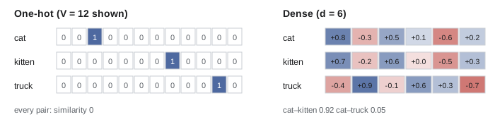
A one-hot vector represents word \(i\) of a vocabulary of size \(V\) as a vector of \(V\) zeros with a single 1 in position \(i\). All one-hot vectors are orthogonal, so every pair of words has similarity zero. A dense embedding instead uses \(d\) dimensions, with \(d\) typically 50 to 1000, far smaller than \(V\), and every dimension is used by every word. An embedding matrix \(E\) of shape \(V \times d\) stores one row per word; multiplying a one-hot vector by \(E\) simply selects that word's row, which is why embedding layers are implemented as table lookups.

Count-based embeddings

The direct way to apply the distributional hypothesis is to count. A word-context co-occurrence matrix \(C\) has one row per word and one column per context word, with \(C_{wc}\) the number of times \(c\) appears within a window (say two words either side) of \(w\). Raw counts are dominated by frequent words such as "the", so they are reweighted by pointwise mutual information (PMI), which compares how often two words occur together with how often they would if they were independent:

PMI is positive when the words co-occur more than chance, zero when independent, and negative when they avoid each other. Negative values are unreliable for rare pairs, so positive PMI (PPMI) replaces them with zero. The resulting matrix is still \(V \times V\) and sparse; a truncated singular value decomposition (AI-210) keeps the top \(k\) singular vectors, giving \(k\)-dimensional dense vectors. This approach, known as latent semantic analysis when applied to word-document matrices, captures the main patterns of co-occurrence in a few dimensions.

import numpy as np

rng = np.random.default_rng(0)
animals = ["cat", "dog", "horse", "cow"]
vehicles = ["car", "truck", "bus", "van"]
foods = ["bread", "rice", "apple", "cheese"]
templates = [("the", "A", "ate", "the", "F"), ("the", "A", "slept", "in", "the", "barn"),
             ("she", "drove", "the", "V", "to", "town"), ("the", "V", "needs", "fuel"),
             ("we", "cooked", "the", "F", "for", "dinner"), ("the", "F", "was", "fresh")]
fill = {"A": animals, "V": vehicles, "F": foods}
corpus = []
for _ in range(3000):
    t = templates[rng.integers(len(templates))]
    corpus.append([str(rng.choice(fill[w])) if w in fill else w for w in t])

vocab = sorted({w for s in corpus for w in s})
ix = {w: i for i, w in enumerate(vocab)}
C = np.zeros((len(vocab), len(vocab)))
for s in corpus:                               # window of 2 words each side
    for i, w in enumerate(s):
        for j in range(max(0, i - 2), min(len(s), i + 3)):
            if j != i:
                C[ix[w], ix[s[j]]] += 1

total = C.sum()
pw = C.sum(axis=1, keepdims=True) / total
pc = C.sum(axis=0, keepdims=True) / total
with np.errstate(divide="ignore"):
    pmi = np.log((C / total) / (pw * pc))
ppmi = np.maximum(pmi, 0)

U, S, Vt = np.linalg.svd(ppmi)
k = 5
E = U[:, :k] * S[:k]                           # 5-dimensional word vectors
E /= np.linalg.norm(E, axis=1, keepdims=True)

print("vocabulary:", len(vocab), " co-occurrence matrix:", C.shape, " vectors:", E.shape)
for w in ["cat", "truck", "rice", "ate"]:
    sims = E @ E[ix[w]]
    best = [vocab[i] for i in np.argsort(-sims) if vocab[i] != w][:3]
    print(f"{w:6s} nearest: {best}")
print("cos(cat, dog) =", round(float(E[ix["cat"]] @ E[ix["dog"]]), 2),
      "  cos(cat, truck) =", round(float(E[ix["cat"]] @ E[ix["truck"]]), 2))

vocabulary: 29  co-occurrence matrix: (29, 29)  vectors: (29, 5)
cat    nearest: ['cow', 'horse', 'dog']
truck  nearest: ['bus', 'van', 'car']
rice   nearest: ['bread', 'cheese', 'apple']
ate    nearest: ['the', 'cooked', 'in']
cos(cat, dog) = 1.0   cos(cat, truck) = 0.02

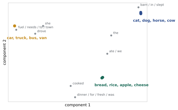
The corpus was generated from templates in which animals eat and sleep, vehicles are driven and need fuel, and food is cooked and eaten. Nothing told the method about these categories, yet with only five dimensions each word's nearest neighbors are the other members of its category: the animals share contexts like "ate" and "barn", the vehicles share "drove" and "fuel". The cosine similarity of "cat" and "dog" rounds to 1.0 because in this artificial corpus they appear in exactly the same kinds of contexts, while "cat" and "truck" are nearly orthogonal. Verbs such as "ate" have less clear neighbors because each occupies its own slot in the templates.

Predictive embeddings: word2vec

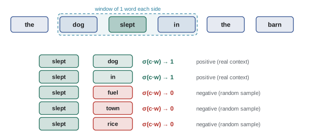
In 2013, Mikolov and colleagues at Google introduced word2vec, which learns embeddings by training a simple model to predict context, rather than counting. The skip-gram variant predicts each context word from the center word; the continuous bag-of-words (CBOW) variant predicts the center word from the average of its context. Skip-gram with negative sampling (SGNS) keeps two vectors per word, a target vector \(\mathbf{w}\) and a context vector \(\mathbf{c}\), and trains a logistic classifier to tell real (word, context) pairs from random "negative" pairs:

where \(\sigma(x) = 1/(1 + e^{-x})\) and the \(K\) negative words (typically 5 to 20) are sampled from the unigram distribution raised to the 3/4 power, which samples rare words a little more often than their frequency. Minimizing this loss pushes the target vector toward the vectors of words that really appear near it and away from random words. Because each update touches only \(K + 1\) context vectors instead of the whole vocabulary, training is fast enough to process billions of words. Other refinements include subsampling very frequent words and dynamic window sizes.

import numpy as np

rng = np.random.default_rng(1)
animals = ["cat", "dog", "horse", "cow"]
vehicles = ["car", "truck", "bus", "van"]
foods = ["bread", "rice", "apple", "cheese"]
templates = [("the", "A", "ate", "the", "F"), ("the", "A", "slept", "in", "the", "barn"),
             ("she", "drove", "the", "V", "to", "town"), ("the", "V", "needs", "fuel"),
             ("we", "cooked", "the", "F", "for", "dinner"), ("the", "F", "was", "fresh")]
fill = {"A": animals, "V": vehicles, "F": foods}
corpus = [[str(rng.choice(fill[w])) if w in fill else w for w in templates[rng.integers(6)]]
          for _ in range(3000)]
vocab = sorted({w for s in corpus for w in s})
ix = {w: i for i, w in enumerate(vocab)}
pairs = [(ix[s[i]], ix[s[j]]) for s in corpus for i in range(len(s))
         for j in range(max(0, i - 2), min(len(s), i + 3)) if j != i]
counts = np.bincount([c for _, c in pairs], minlength=len(vocab)).astype(float)
noise = counts ** 0.75; noise /= noise.sum()      # negative-sampling distribution

d, K, lr = 10, 5, 0.025
W = rng.normal(0, 0.1, (len(vocab), d))           # target (input) vectors
Cv = np.zeros((len(vocab), d))                    # context (output) vectors
sig = lambda x: 1 / (1 + np.exp(-x))

order = np.concatenate([rng.permutation(len(pairs)) for _ in range(2)])
block = len(order) // 6
loss = 0.0
for step, n in enumerate(order, 1):
    t, c = pairs[n]
    negs = rng.choice(len(vocab), K, p=noise)
    ctx = np.concatenate(([c], negs))
    label = np.zeros(K + 1); label[0] = 1
    s = sig(Cv[ctx] @ W[t])
    g = s - label                                  # gradient of logistic loss
    loss -= np.log(s[0] + 1e-9) + np.log(1 - s[1:] + 1e-9).sum()
    gw = g @ Cv[ctx]
    Cv[ctx] -= lr * np.outer(g, W[t])
    W[t] -= lr * gw
    if step % block == 0:
        print(f"after {step:6d} pairs: mean loss {loss / block:.3f}")
        loss = 0.0

E = W / np.linalg.norm(W, axis=1, keepdims=True)
for w in ["dog", "bus", "cheese"]:
    sims = E @ E[ix[w]]
    print(f"{w:7s}", [vocab[i] for i in np.argsort(-sims)[1:4]])

after  14752 pairs: mean loss 2.595
after  29504 pairs: mean loss 1.994
after  44256 pairs: mean loss 1.953
after  59008 pairs: mean loss 1.974
after  73760 pairs: mean loss 1.985
after  88512 pairs: mean loss 2.008
dog     ['cow', 'cat', 'horse']
bus     ['van', 'car', 'truck']
cheese  ['rice', 'bread', 'apple']

The loss falls quickly in the first block of training pairs and then levels off around 2.0; it cannot fall to zero, because many words share contexts and the negative samples sometimes include true context words. The learned target vectors again place each word near the other members of its category. Levy and Goldberg showed in 2014 that SGNS implicitly factorizes a shifted PMI matrix, so count-based and predictive methods are closer than they appear; in practice, careful tuning matters as much as the choice of method.

Two other influential methods followed. GloVe (Stanford, 2014) fits word vectors so that their dot products match the logarithms of global co-occurrence counts, combining count statistics with an efficient learned model. fastText (Facebook, 2016) represents each word as the sum of vectors for its character n-grams (for example "<wh", "whe", "her", "ere", "re>" for "where"), so it can build vectors for unseen and misspelled words and works well for languages with rich morphology.

What embeddings capture

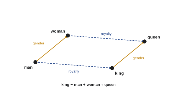
Well-trained embeddings encode surprisingly regular relationships. Famously, the vector \(\mathbf{v}_{king} - \mathbf{v}_{man} + \mathbf{v}_{woman}\) is closer to \(\mathbf{v}_{queen}\) than to any other word, and similar offsets capture country-capital, verb tense and plural relationships. These analogies work because a consistent difference in contexts (such as the contexts that distinguish male and female words) corresponds to a consistent direction in the vector space.

Analogy results have been overstated: they depend on excluding the input words, work for some relation types far better than others, and partly reflect simple frequency effects. Embeddings are better evaluated on downstream tasks and on word-similarity benchmarks that compare cosine similarity with human ratings. Static embeddings also have a fundamental limitation: each word type has one vector, so "bank" (river) and "bank" (money) share a single vector that blends both meanings.

Bias in embeddings

Because embeddings learn from human-written text, they absorb the associations in that text, including social stereotypes. In 2016, Bolukbasi and colleagues showed that word2vec vectors trained on news text completed "man is to computer programmer as woman is to ?" with "homemaker", and that occupation words lay along a gender direction in proportion to stereotypes. The Word Embedding Association Test (WEAT) measures such associations statistically and has found biases related to gender, race, age and other attributes that mirror findings from human implicit association tests.

These biases matter when embeddings feed real decisions, such as ranking job applicants, moderating content or retrieving documents. Proposed mitigations include identifying a bias direction (for example the average of \(\mathbf{v}_{she} - \mathbf{v}_{he}\) over several word pairs) and projecting it out of words that should be neutral, rebalancing training data, and testing downstream systems for disparate outcomes. Later research showed that projection methods mostly hide bias rather than remove it, since the associations remain recoverable from other directions. The more reliable lesson is to measure bias in the final application, on the decisions that matter, rather than assuming a debiased representation makes a system fair.

From static to contextual embeddings

Static embeddings give each word one vector regardless of context. Contextual embeddings instead compute a different vector for each occurrence of a word, depending on the surrounding sentence. ELMo (2018) produced them from a bidirectional LSTM language model (Lesson 4); BERT (2018) from a transformer encoder (Lesson 6). In "she sat by the river bank" and "the bank approved the loan", a contextual model gives "bank" different vectors that cluster with other river words and other financial words respectively.

Today, embeddings are used in two main ways. Within language models, the input embedding layer maps tokens to vectors that the transformer layers then contextualize. Separately, sentence and document embedding models (such as Sentence-BERT and the embedding models offered by AI providers) map a whole passage to a single vector, so that semantic search can find passages similar in meaning to a query even without shared words. These vectors are stored in vector databases and searched with approximate nearest-neighbor algorithms, forming the retrieval half of retrieval-augmented generation (Lesson 9 and AI-410).

Lesson 3 puts these representations to work in classifiers and taggers, and Lesson 9 returns to sentence embeddings for retrieval.