Text, tokens and representations

Natural language processing (NLP) is the study of how computers can analyze, understand and generate human language. It powers search engines, translation, spam filters, voice assistants, document classification and, most visibly, large language models such as the chat assistants that became widespread after 2022. Every NLP system faces the same first problem: text is a sequence of characters, while machine learning models need numbers. This lesson covers how raw text is cleaned and split into tokens, how modern subword tokenizers work, how documents can be represented as vectors of word counts, and how the simplest language models assign probabilities to sentences. These ideas remain at the heart of modern systems: every large language model begins with a tokenizer and is trained to do exactly what an n-gram model does, predict the next token, only far better. The section at the end of this lesson shows how the twelve lessons of the course fit together.

Characters, Unicode and normalization

Computers store text as sequences of code points defined by the Unicode standard, which covers over 150,000 characters from almost every writing system, plus symbols and emoji. Unicode text is usually stored in the UTF-8 encoding, which uses 1 byte for ASCII characters and 2 to 4 bytes for others. Several complications arise before any modeling begins:

• The same visible text can have different encodings: "é" can be one code point or "e" plus a combining accent. Unicode normalization (NFC or NFKC) converts text to a standard form so that identical-looking strings compare equal.
• Case: lowercasing ("case folding") merges "The" and "the" but loses information such as proper nouns ("Apple" the company) and acronyms ("US" versus "us").
• Whitespace, punctuation and markup: text scraped from the web contains HTML, repeated spaces, line breaks and boilerplate that must be cleaned.
• Languages without spaces: Chinese, Japanese and Thai do not separate words with spaces, so word segmentation is itself a learning problem.

Classical pipelines often also removed stop words (very common words such as "the" and "of") and applied stemming (cutting words to a stem, "running" to "run") or lemmatization (mapping to a dictionary form, "better" to "good"). Modern neural models usually skip these steps, because they discard information the model can use.

Tokenization

Tokenization splits text into units called tokens. The simplest approach treats each run of letters and digits as a word and each punctuation mark as a separate token. The number of tokens is the text's length; the number of distinct tokens is the number of types, or the vocabulary size.

from collections import Counter

text = """The cat sat on the mat. The dog sat on the log.
The cat chased the dog, and the dog chased the cat!
Cats and dogs are not the same; a cat is a cat."""

def tokenize(s):
    # split into words and single punctuation marks without regular expressions
    tokens, word = [], ""
    for ch in s:
        if ch.isalnum():
            word += ch
        else:
            if word:
                tokens.append(word)
                word = ""
            if not ch.isspace():
                tokens.append(ch)
    if word:
        tokens.append(word)
    return tokens

raw = tokenize(text)
norm = [t.lower() for t in raw if t.isalnum()]
print("tokens:", len(raw), " word tokens:", len(norm), " types:", len(set(norm)))
print("first 12:", raw[:12])
counts = Counter(norm)
for rank, (w, c) in enumerate(counts.most_common(6), 1):
    print(f"rank {rank}: {w:6s} count {c:2d}  rank*count {rank * c}")

tokens: 41  word tokens: 35  types: 16
first 12: ['The', 'cat', 'sat', 'on', 'the', 'mat', '.', 'The', 'dog', 'sat', 'on', 'the']
rank 1: the    count  9  rank*count 9
rank 2: cat    count  5  rank*count 10
rank 3: dog    count  3  rank*count 9
rank 4: sat    count  2  rank*count 8
rank 5: on     count  2  rank*count 10
rank 6: chased count  2  rank*count 12

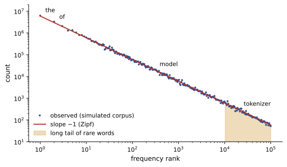
Even in this three-sentence text, the most common word ("the") occurs far more often than most others, and half the types occur once or twice. In large corpora this pattern follows Zipf's law: the frequency of the word of rank \(r\) is roughly proportional to \(1/r\), so rank times count is roughly constant. Our tiny sample shows the product hovering around 10. Zipf's law has a crucial consequence: no matter how much text a model sees, new text keeps containing words it has never seen before. A word-level vocabulary of 50,000 words still meets unknown names, misspellings, numbers, technical terms and new coinages, which classical systems mapped to a single <unk> token, losing their meaning.

Subword tokenization

Subword tokenizers split text into pieces that are smaller than words but larger than characters. Frequent words become single tokens; rare words are broken into meaningful pieces ("unbelievably" into "un", "believ", "ably"); and any string, however unusual, can be represented because the pieces include single characters or bytes. Three algorithms dominate:

• Byte-pair encoding (BPE): start with characters and repeatedly merge the most frequent adjacent pair into a new symbol, until the vocabulary reaches a chosen size. Used, in its byte-level form, by GPT models and many others.
• WordPiece: similar merging, but choosing merges that most increase the likelihood of the training data. Used by BERT.
• Unigram language model (in the SentencePiece library): start with a large vocabulary and prune pieces that contribute least to the likelihood; tokenization chooses the most probable segmentation. SentencePiece treats spaces as ordinary symbols, so it works for languages without spaces.

from collections import Counter

corpus = {"low": 5, "lower": 2, "newest": 6, "widest": 3}
# each word is a tuple of symbols ending with an end-of-word marker
vocab = {tuple(w) + ("_",): c for w, c in corpus.items()}

def pair_counts(vocab):
    pairs = Counter()
    for word, c in vocab.items():
        for a, b in zip(word, word[1:]):
            pairs[(a, b)] += c
    return pairs

def merge(vocab, pair):
    out = {}
    for word, c in vocab.items():
        w, i = [], 0
        while i < len(word):
            if i < len(word) - 1 and (word[i], word[i + 1]) == pair:
                w.append(word[i] + word[i + 1]); i += 2
            else:
                w.append(word[i]); i += 1
        out[tuple(w)] = c
    return out

merges = []
for step in range(8):
    pairs = pair_counts(vocab)
    best = max(pairs, key=lambda p: (pairs[p], p))
    merges.append(best)
    vocab = merge(vocab, best)
    print(f"merge {step + 1}: {best[0]} + {best[1]} -> {best[0] + best[1]}  (count {pairs[best]})")

def encode(word):
    w = list(word) + ["_"]
    for a, b in merges:
        i, out = 0, []
        while i < len(w):
            if i < len(w) - 1 and w[i] == a and w[i + 1] == b:
                out.append(a + b); i += 2
            else:
                out.append(w[i]); i += 1
        w = out
    return w

for word in ["lowest", "newer", "wider"]:
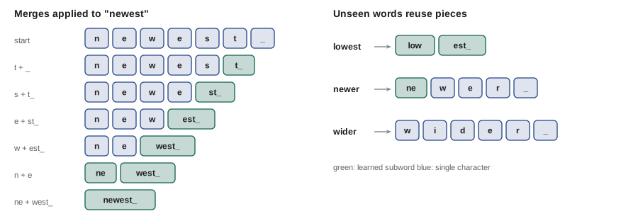
    print(word, "->", encode(word))

merge 1: t + _ -> t_  (count 9)
merge 2: s + t_ -> st_  (count 9)
merge 3: e + st_ -> est_  (count 9)
merge 4: o + w -> ow  (count 7)
merge 5: l + ow -> low  (count 7)
merge 6: w + est_ -> west_  (count 6)
merge 7: n + e -> ne  (count 6)
merge 8: ne + west_ -> newest_  (count 6)
lowest -> ['low', 'est_']
newer -> ['ne', 'w', 'e', 'r', '_']
wider -> ['w', 'i', 'd', 'e', 'r', '_']

The learned merges reflect the corpus: the frequent ending "est" (from "newest" and "widest") becomes a unit early, and "low" becomes a token. The unseen word "lowest" is split into two learned pieces, "low" and "est_", while "newer" and "wider" fall back mostly to characters because their endings were rare in training. With tens of thousands of merges learned from billions of words, common words become single tokens and rare words split into a few meaningful pieces. Byte-level BPE starts from the 256 possible byte values instead of characters, so it never encounters an unknown symbol, including emoji and any script.

Vocabulary size is a trade-off. A larger vocabulary makes sequences shorter (fewer tokens per word, so faster processing and more text fits in a model's context window) but enlarges the embedding and output layers and leaves rare tokens poorly trained. Modern models use roughly 32,000 to 260,000 tokens. Tokenizers trained mostly on English text split other languages into more tokens per word, which makes the same content more expensive to process and leaves less room in the context window, a fairness issue for multilingual applications.

In the US this matters for the roughly 13% of residents who speak Spanish at home and for many other language communities: federal agencies and recipients of federal funds have obligations to provide meaningful access to people with limited English proficiency, and many states have their own language-access laws. Indigenous languages such as Navajo, Cherokee (with its own syllabary) and Yupik have very little digital text, so tokenizers and models serve them poorly unless built with community partners. Checking tokens per word and model quality in each language should be part of any deployment that serves multilingual users.

Bag of words and TF-IDF

The simplest way to turn a document into a vector is the bag of words: one dimension per vocabulary word, with the count of that word in the document, ignoring order. "The dog bit the man" and "the man bit the dog" have the same bag of words, which shows what is lost, but for many tasks such as topic classification and search, word counts carry most of the useful signal.

Raw counts overweight common words. TF-IDF (term frequency times inverse document frequency) weights each word by how rare it is across documents:

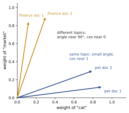
where \(\text{tf}(w,d)\) is the count of word \(w\) in document \(d\), \(N\) is the number of documents and \(\text{df}(w)\) is the number of documents containing \(w\). A word in every document gets weight \(\log 1 = 0\); a word in one document gets the largest weight. Libraries often add 1 to the idf so common words are not completely ignored. Documents are then compared with cosine similarity, the cosine of the angle between their vectors, which ignores document length:

import numpy as np

docs = ["the cat sat on the mat",
        "the dog sat on the log",
        "cats and dogs make good pets",
        "the stock market fell sharply today",
        "markets rallied as stocks rose"]
toks = [d.split() for d in docs]
vocab = sorted({w for t in toks for w in t})
idx = {w: i for i, w in enumerate(vocab)}

tf = np.zeros((len(docs), len(vocab)))
for d, t in enumerate(toks):
    for w in t:
        tf[d, idx[w]] += 1
df = (tf > 0).sum(axis=0)
idf = np.log(len(docs) / df) + 1          # smoothed idf, as in many libraries
tfidf = tf * idf
tfidf /= np.linalg.norm(tfidf, axis=1, keepdims=True)

print("vocabulary size:", len(vocab))
print("idf(the) =", round(idf[idx["the"]], 2), "  idf(cat) =", round(idf[idx["cat"]], 2))
sim = tfidf @ tfidf.T
np.set_printoptions(precision=2, suppress=True)
print(sim)

q = "stock markets"
v = np.zeros(len(vocab))
for w in q.split():
    if w in idx:
        v[idx[w]] += idf[idx[w]]
print("query:", q, "-> scores", (tfidf @ (v / np.linalg.norm(v))).round(2))

vocabulary size: 23
idf(the) = 1.51   idf(cat) = 2.61
[[1.   0.55 0.   0.14 0.  ]
 [0.55 1.   0.   0.14 0.  ]
 [0.   0.   1.   0.   0.  ]
 [0.14 0.14 0.   1.   0.  ]
 [0.   0.   0.   0.   1.  ]]
query: stock markets -> scores [0.   0.   0.   0.31 0.32]

The two pet sentences are similar (0.55) because they share "sat", "on" and "the", but "cats and dogs make good pets" has zero similarity to "the cat sat on the mat": to a bag of words, "cat" and "cats" are unrelated symbols. Likewise the query "stock markets" matches "stock" in one finance document and "markets" in the other, but cannot tell that "stocks" and "stock" mean the same thing. This sparsity, where related words share no dimensions, is the motivation for the dense word embeddings of Lesson 2. Even so, TF-IDF and its refinement BM25 (Lesson 12) remain strong baselines for search and are still used in retrieval systems alongside neural methods.

N-gram language models

A language model assigns a probability to a sequence of tokens. By the chain rule of probability, any sequence probability can be written as a product of next-token probabilities:

An n-gram model makes the Markov assumption that each token depends only on the previous \(n-1\) tokens. A bigram model uses \(P(w_i \mid w_{i-1})\), estimated by maximum likelihood as a ratio of counts:

Sentences are padded with start and end markers, <s> and </s>, so the model also learns how sentences begin and end. Any bigram not seen in training gets probability zero, which makes the probability of any test sentence containing it zero. Smoothing reserves probability for unseen events. Add-k smoothing adds \(k\) to every count:

where \(V\) is the number of possible next tokens. Better methods such as Kneser-Ney smoothing, which back off to lower-order models and account for how many different contexts a word appears in, powered speech recognition and machine translation until neural models replaced them.

Language models are evaluated by perplexity, the exponential of the average negative log probability per token on held-out text:

Perplexity can be read as the effective number of equally likely choices the model is deciding among at each step. A model that predicts uniformly over 10,000 words has perplexity 10,000; a good model of English has perplexity in the tens or lower. Lower is better, and perplexity is directly related to the cross-entropy loss used to train neural language models (AI-210).

import math
from collections import Counter

train = ["the cat sat on the mat", "the dog sat on the log", "the cat saw the dog",
         "a dog sat on a mat", "the cat ate", "a cat sat"]
test = ["the dog sat on the mat", "a cat saw a dog"]

def pad(s):
    return ["<s>"] + s.split() + ["</s>"]

uni, bi = Counter(), Counter()
for s in train:
    t = pad(s)
    uni.update(t[:-1])
    bi.update(zip(t[:-1], t[1:]))
V = len({w for s in train for w in pad(s)}) - 1      # possible next tokens (exclude <s>)

def prob(prev, w, k):
    return (bi[(prev, w)] + k) / (uni[prev] + k * V)

def perplexity(sents, k):
    logp, n = 0.0, 0
    for s in sents:
        t = pad(s)
        for prev, w in zip(t[:-1], t[1:]):
            p = prob(prev, w, k)
            if p == 0:
                return float("inf")
            logp += math.log(p); n += 1
    return math.exp(-logp / n)

print("vocabulary (next-token choices):", V)
print("P(cat | the) MLE =", round(prob("the", "cat", 0), 3))
for k in (0, 0.01, 0.1, 1.0):
    print(f"k = {k:<5} train PPL {perplexity(train, k):6.2f}   test PPL {perplexity(test, k):6.2f}")

vocabulary (next-token choices): 11
P(cat | the) MLE = 0.429
k = 0     train PPL   2.12   test PPL    inf
k = 0.01  train PPL   2.18   test PPL   3.29
k = 0.1   train PPL   2.65   test PPL   3.39
k = 1.0   train PPL   5.29   test PPL   5.94

Without smoothing (\(k = 0\)), the model fits the training data best but assigns zero probability to the test sentence "a cat saw a dog", because "saw a" never occurred in training, so test perplexity is infinite. A small \(k\) gives finite test perplexity; too large a \(k\) spreads probability too evenly and hurts both. The gap between training and test perplexity is a measure of overfitting, exactly as in other machine learning.

N-gram models capture local patterns but cannot use context more than a few words back, need enormous tables of counts (the number of possible 5-grams is astronomical), and cannot generalize from "the cat sat" to "the kitten sat" because words are separate symbols. Neural language models address all three problems: they represent words as dense vectors (Lesson 2), process long contexts with recurrent networks (Lesson 4) or attention (Lesson 6), and share statistical strength across similar words.

How this course is organized

The twelve lessons build from raw text to modern language model systems:

• Lesson 1 (this lesson): text, Unicode, tokenization, bag-of-words representations and n-gram language models.
• Lesson 2: word embeddings, from co-occurrence counts to word2vec and contextual vectors.
• Lesson 3: text classification and sequence labeling, from naive Bayes to BIO tagging with Viterbi decoding.
• Lesson 4: sequence models: recurrent networks, LSTMs, encoder-decoders and decoding.
• Lesson 5: machine translation, beam search and the BLEU and chrF metrics.
• Lesson 6: attention and the transformer.
• Lesson 7: pretrained language models (BERT, GPT, T5), pretraining data and scaling laws.
• Lesson 8: large language models: post-training, prompting, reasoning, decoding and hallucination.
• Lesson 9: dense retrieval and retrieval-augmented generation.
• Lesson 10: efficient NLP: LoRA, quantization, distillation and fast inference.
• Lesson 11: information extraction, question answering and agents.
• Lesson 12: evaluation, applications, risks and the rules that apply to NLP systems.