Non-convex landscapes and training dynamics

The loss of a neural network is a non-convex function of its parameters, with symmetries, saddle points and many minima. Classical optimization theory offers few guarantees for such functions, yet gradient methods train networks with billions of parameters reliably. This lesson looks at what is known about why: the geometry of high-dimensional loss landscapes, the curvature that gradient descent experiences and adapts to, the initialization and architecture choices that keep gradients usable through many layers, numerical precision, and the empirical regularities, from double descent to scaling laws, that guide practice.

Saddle points and local minima

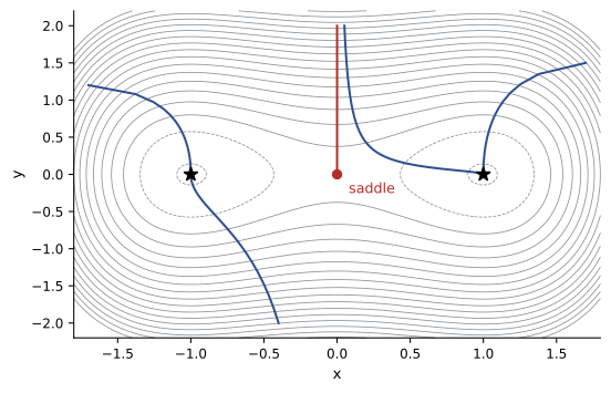
A stationary point (zero gradient) is a minimum if the Hessian is positive definite there, a maximum if negative definite, and a saddle if it has eigenvalues of both signs. In one or two dimensions, poor local minima are the familiar picture of non-convex optimization. In high dimensions the picture changes: for a stationary point to be a minimum, every one of millions of Hessian eigenvalues must be positive, while a saddle needs only one negative. Analyses of random functions and empirical studies of neural networks suggest that most stationary points at high loss are saddles, and that the minima found in large, overparameterized networks tend to have similar, low loss. Separate minima found from different random initializations can often be connected by paths along which the loss stays low (mode connectivity).

Saddles slow gradient descent, because the gradient is small near them, but they rarely trap it: an exact saddle is unstable, and any component of the iterate along a negative-curvature direction grows exponentially. Gradient noise from minibatches helps by supplying such components.

import numpy as np

# f(x, y) = x^4/4 - x^2/2 + y^2/2 : saddle at (0, 0), minima at (+1, 0) and (-1, 0)
grad = lambda w: np.array([w[0] ** 3 - w[0], w[1]])
f = lambda w: w[0] ** 4 / 4 - w[0] ** 2 / 2 + w[1] ** 2 / 2

def descend(w0, noise=0.0, steps=200, eta=0.1, seed=0):
    rng = np.random.default_rng(seed)
    w = np.array(w0, dtype=float)
    for k in range(steps):
        w -= eta * (grad(w) + noise * rng.normal(size=2))
    return w

for start in [(0.0, 2.0), (1e-6, 2.0), (-0.5, 1.0), (2.0, -1.0)]:
    w = descend(start)
    print(f"start {str(start):13s} -> ({w[0]:+.3f}, {w[1]:+.3f}),  f = {f(w):+.3f}")
w = descend((0.0, 2.0), noise=0.01)
print(f"start (0.0, 2.0) with gradient noise -> ({w[0]:+.3f}, {w[1]:+.3f}),  f = {f(w):+.3f}")

start (0.0, 2.0)    -> (+0.000, +0.000),  f = +0.000
start (1e-06, 2.0)  -> (+1.000, +0.000),  f = -0.250
start (-0.5, 1.0)   -> (-1.000, +0.000),  f = -0.250
start (2.0, -1.0)   -> (+1.000, -0.000),  f = -0.250
start (0.0, 2.0) with gradient noise -> (+0.999, +0.001),  f = -0.250

Curvature during training

The Hessian of a trained network has a characteristic spectrum: a large bulk of eigenvalues near zero, reflecting many directions in which the loss barely changes (redundancy in an overparameterized model), and a small number of large outlier eigenvalues, often roughly as many as there are classes. The largest eigenvalue, the sharpness \(\lambda_{\max}\), determines the stable learning rate, as on a quadratic: gradient descent is stable only when \(\eta < 2/\lambda_{\max}\).

Experiments by Cohen and colleagues (2021) found something unexpected about full-batch gradient descent on neural networks. Sharpness rises during training (progressive sharpening) until it reaches about \(2/\eta\), and then, instead of diverging, training continues at the edge of stability: the sharpness hovers around \(2/\eta\), the loss decreases non-monotonically over the long run with short-term oscillations, and the network moves into regions just flat enough for the chosen learning rate. In effect, the learning rate selects the curvature of the solution. Similar but noisier behavior occurs with SGD and Adam.

Sharp and flat minima

Flat minima, where the loss rises slowly in most directions, have long been associated with better generalization: a small shift between the training and test distributions changes the loss little. The noise of small-batch SGD and large learning rates both bias training toward flatter regions, which is one reason they often generalize well. Sharpness-aware minimization (SAM) makes the preference explicit by minimizing the worst-case loss in a small neighborhood of the parameters. The relationship is not simple, however: sharpness depends on the parameterization (rescaling the weights of a ReLU network changes it without changing the function), so it is a heuristic rather than a law.

Initialization

A deep network multiplies its input by many weight matrices. If each layer scales the signal's variance by a factor slightly above or below one, the signal explodes or vanishes exponentially with depth, and so do the gradients flowing backward, making training impossible. Initialization schemes choose the scale of random initial weights to keep variances roughly constant:

• Xavier (Glorot) initialization, for tanh or linear layers: weights with variance \(2/(n_{\text{in}} + n_{\text{out}})\), balancing the forward and backward passes.
• He (Kaiming) initialization, for ReLU layers: variance \(2/n_{\text{in}}\), where the factor 2 compensates for ReLU zeroing half of its inputs.

import numpy as np

rng = np.random.default_rng(0)
width, depth = 256, 30
x = rng.normal(size=(1000, width))

def forward_stds(scale_fn, act):
    h, stds = x, []
    for _ in range(depth):
        W = rng.normal(size=(width, width)) * scale_fn(width)
        h = act(h @ W)
        stds.append(h.std())
    return stds

relu = lambda z: np.maximum(z, 0)
cases = {
    "ReLU, std 0.01": (lambda n: 0.01, relu),
    "ReLU, He sqrt(2/n)": (lambda n: np.sqrt(2 / n), relu),
    "ReLU, std 0.1": (lambda n: 0.1, relu),
    "tanh, Xavier sqrt(1/n)": (lambda n: np.sqrt(1 / n), np.tanh),
}
print("activation std at layer:      1          10          30")
for name, (s, a) in cases.items():
    st = forward_stds(s, a)
    print(f"{name:24s} {st[0]:10.2e}  {st[9]:10.2e}  {st[29]:10.2e}")

activation std at layer:      1          10          30
ReLU, std 0.01             9.40e-02    3.04e-10    5.06e-29
ReLU, He sqrt(2/n)         8.26e-01    8.65e-01    6.84e-01
ReLU, std 0.1              9.33e-01    2.73e+00    2.79e+01
tanh, Xavier sqrt(1/n)     6.27e-01    2.31e-01    1.27e-01

Too small a scale makes the signal vanish to nothing within a few layers, too large makes it explode, and the He scale keeps it steady through all 30 layers. (With width 256, the He standard deviation is \(\sqrt{2/256} = 0.088\), so 0.1 is only slightly too large, yet the effect compounds to a large growth over 30 layers.) With tanh, Xavier scaling lets the signal shrink only slowly, from 0.63 to 0.13 over 30 layers, because tanh compresses large values; normalization layers (below) remove the remaining drift.

Architecture for trainability

Initialization alone is not enough for very deep networks, because the weights change during training. Two architectural ideas made deep networks reliably trainable:

• Residual connections compute \(\mathbf{h}_{l+1} = \mathbf{h}_l + F(\mathbf{h}_l)\): each block adds a correction to an identity path. Gradients flow back along the identity path undiminished, so networks of hundreds of layers train. Residual connections are part of essentially every modern architecture, including transformers.
• Normalization layers rescale activations to a standard mean and variance. Batch normalization normalizes over the examples in a minibatch and was decisive for convolutional networks; layer normalization normalizes over the features of each example and is standard in transformers. Normalization makes the loss less sensitive to the scale of the weights, allowing larger learning rates.

Even with these, the training of very large models is punctuated by loss spikes: sudden jumps in the loss, sometimes recovering and sometimes diverging. Common remedies are gradient clipping, learning rate warmup, lower Adam \(\beta_2\), normalizing queries and keys in attention, skipping batches that produce anomalous gradients, and restarting from a checkpoint before the spike with a lower learning rate.

Numerical precision

Large models are trained in reduced precision to save memory and time. The two 16-bit formats differ in what they sacrifice: IEEE half precision (FP16) has 10 mantissa bits but only 5 exponent bits, so its smallest normal number is about \(6.1 \times 10^{-5}\) and its largest is 65,504; bfloat16 (BF16) has only 7 mantissa bits but the same 8 exponent bits as FP32, so it covers the same range with less precision. Small gradients underflow to zero in FP16; mixed-precision training with FP16 therefore uses loss scaling, multiplying the loss by a large factor before backpropagation so that gradients fall within range, then dividing the gradients before the update. BF16 usually needs no loss scaling, which is why it has become standard on accelerators that support it. In both cases a 32-bit master copy of the weights accumulates the small updates.

import numpy as np

grads = np.array([3e-3, 2e-5, 4e-7, 6e-9], dtype=np.float32)
print("FP32 gradients:        ", grads)
print("cast to FP16:          ", grads.astype(np.float16).astype(np.float32))
scale = 65536.0
scaled = (grads * scale).astype(np.float16)                # backprop in FP16 with scaled loss
print("FP16 with loss scaling:", scaled.astype(np.float32) / scale)

w = np.float16(1.0)
print("FP16 weight 1.0 + update 1e-4 =", w + np.float16(1e-4), "(update lost: needs FP32 master weights)")

FP32 gradients:         [3.e-03 2.e-05 4.e-07 6.e-09]
cast to FP16:           [3.0002594e-03 2.0027161e-05 4.1723251e-07 0.0000000e+00]
FP16 with loss scaling: [3.0002594e-03 1.9997358e-05 4.0000305e-07 5.9990271e-09]
FP16 weight 1.0 + update 1e-4 = 1.0 (update lost: needs FP32 master weights)

Overparameterization, double descent and implicit bias

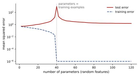
Classical statistics predicts that a model with more parameters than training examples will overfit. Modern networks routinely have far more parameters than examples, fit their training data perfectly, and still generalize. Plotting test error against model size often shows double descent: error falls, rises to a peak near the interpolation threshold, where the model has just enough capacity to fit the training data exactly, and then falls again as the model grows further. Past the threshold there are many parameter settings that fit the data, and the optimizer's implicit bias determines which one is found. For linear least squares, gradient descent started at zero converges to the minimum-norm interpolating solution; for deep networks, the implicit biases of SGD, its learning rate and noise, and the architecture together favor solutions that generalize.

Scaling laws and training at scale

For large language models, test loss has been found to fall smoothly as a power law in model size, data and compute over many orders of magnitude. These scaling laws let teams predict the loss of a large model from small experiments, and choose how to divide a compute budget between parameters and data. A widely cited analysis (Hoffmann and colleagues, 2022, the "Chinchilla" study) found that, for a fixed compute budget, loss is minimized by scaling parameters and training tokens roughly in proportion, at about 20 tokens per parameter; training compute is about \(6ND\) floating-point operations for \(N\) parameters and \(D\) tokens. Many current models are trained on far more tokens than that, accepting extra training compute to obtain a smaller model that is cheaper to run.

Finally, a practical tool ties the chapter together: the learning rate range test. Train briefly while increasing the learning rate exponentially from very small to very large, and plot the loss. The loss falls slowly at first, then rapidly, then becomes unstable and rises; a good peak learning rate lies somewhat below the point where the loss is lowest, in the steep part of the curve. It is a quick, empirical way to locate the edge of stability for a new model and data set.

Lesson 10 turns to the hyperparameters that control these dynamics, and Lesson 12 to training at the scale where scaling laws apply.