Convexity, subgradients and optimality

Lesson 1 analyzed gradient descent using two properties of the objective, smoothness and strong convexity, and showed how they control convergence. This lesson steps back to examine those properties directly. Convexity is what makes an optimization problem tractable: every local minimum is global, simple conditions certify optimality, and algorithms come with guarantees. Many machine learning objectives are convex (linear and logistic regression, support vector machines, lasso), and even for non-convex deep networks, convex analysis supplies the vocabulary and the local picture. The lesson also handles functions that are not differentiable, such as absolute values and hinge losses, through subgradients, and ends with conditions that tell when a point is optimal.

Convex sets and functions

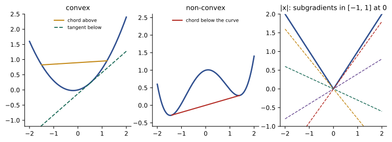
A set \(C\) is convex if the line segment between any two of its points lies in it. A function \(f\) is convex if its domain is convex and, for all \(x, y\) and \(0 \le \theta \le 1\),

so the chord between two points of the graph lies on or above the graph. Equivalent tests are often easier to use:

• First order: if \(f\) is differentiable, it is convex exactly when \(f(y) \ge f(x) + \nabla f(x)^T(y - x)\) for all \(x, y\): every tangent plane is a global under-estimator.
• Second order: if \(f\) is twice differentiable, it is convex exactly when its Hessian \(\nabla^2 f(x)\) is positive semidefinite everywhere.

Building convex functions

Most convex objectives in machine learning are built from a few operations that preserve convexity:

• Nonnegative weighted sums of convex functions (a loss plus a regularizer).
• Composition with an affine map: if \(f\) is convex, so is \(f(Ax + b)\). This is why losses of linear predictions, such as \(\ell(y_i, x_i^T w)\), are convex in \(w\) when \(\ell\) is convex in its second argument.
• Pointwise maximum: the maximum of convex functions is convex (the hinge loss \(\max(0, 1 - y\,x^Tw)\) and the ReLU are examples).
• Norms are convex; so are their squares.

Smoothness and strong convexity revisited

Two constants bracket the curvature of a function and decide how fast first-order methods converge (Lesson 1):

• \(L\)-smoothness: the gradient is \(L\)-Lipschitz, \(\|\nabla f(x) - \nabla f(y)\| \le L\|x - y\|\); for twice-differentiable functions, the Hessian's eigenvalues are at most \(L\). A step size of \(1/L\) is always safe.
• \(\mu\)-strong convexity: \(f(y) \ge f(x) + \nabla f(x)^T(y - x) + \frac{\mu}{2}\|y - x\|^2\); the Hessian's eigenvalues are at least \(\mu > 0\). A strongly convex function has a unique minimizer, and gradient descent converges linearly to it.

The ratio \(\kappa = L/\mu\) is the condition number. Data determine both constants: for least squares, \(L\) and \(\mu\) are the largest and smallest eigenvalues of \(X^TX/n\); for logistic regression, \(L\) is a quarter of the largest, because \(\sigma(1-\sigma) \le 1/4\). Adding an L2 penalty \(\frac{\lambda}{2}\|w\|^2\) adds \(\lambda\) to every eigenvalue, making any convex loss \(\lambda\)-strongly convex.

import numpy as np

rng = np.random.default_rng(0)
n, d = 500, 5
X = rng.normal(size=(n, d)) * np.array([1.0, 2.0, 0.5, 3.0, 1.0])
y = (X @ rng.normal(size=d) + rng.normal(size=n) > 0).astype(float)

def logistic_hessian(w):
    p = 1 / (1 + np.exp(-X @ w))
    return (X.T * (p * (1 - p))) @ X / n

# Convexity: the Hessian is positive semidefinite at every point we try
mins = [np.linalg.eigvalsh(logistic_hessian(rng.normal(size=d) * 3)).min() for _ in range(200)]
print(f"smallest Hessian eigenvalue over 200 random points: {min(mins):.2e} (never negative)")

# Smoothness: L = largest eigenvalue of X^T X / (4 n) bounds the logistic Hessian everywhere
L_log = np.linalg.eigvalsh(X.T @ X / n).max() / 4
print(f"logistic loss smoothness L = {L_log:.3f}; safe step 1/L = {1 / L_log:.3f}")

# Adding an L2 penalty lam/2 ||w||^2 makes it lam-strongly convex
lam = 0.1
H0 = logistic_hessian(np.zeros(d)) + lam * np.eye(d)
ev = np.linalg.eigvalsh(H0)
print(f"with lambda = {lam}: Hessian eigenvalues at w = 0 from {ev.min():.3f} to {ev.max():.3f}")
print(f"global condition number bound kappa = (L + lam) / lam = {(L_log + lam) / lam:.1f}")

smallest Hessian eigenvalue over 200 random points: 3.11e-04 (never negative)
logistic loss smoothness L = 2.390; safe step 1/L = 0.418
with lambda = 0.1: Hessian eigenvalues at w = 0 from 0.155 to 2.490
global condition number bound kappa = (L + lam) / lam = 24.9

Non-differentiable functions and subgradients

Many useful objectives have corners: the absolute value in the lasso and in robust regression, the hinge loss of support vector machines, the maximum in ReLU networks. At a corner the gradient does not exist, but a convex function still has subgradients: vectors \(g\) such that

The set of all subgradients at \(x\) is the subdifferential \(\partial f(x)\). Where \(f\) is differentiable it contains only the gradient; at a corner it contains every slope between the one-sided slopes. For \(|x|\) at 0 it is the interval \([-1, 1]\); for \(\max(0, 1 - z)\) at \(z = 1\) it is \([-1, 0]\).

Subgradients combine like gradients: the subdifferential of a sum is the sum of subdifferentials, and composition with an affine map works through the chain rule \(A^T\partial f(Ax + b)\).

The subgradient method

Replacing the gradient by any subgradient gives the subgradient method, \(x_{k+1} = x_k - \eta_k g_k\). Unlike gradient descent, it is not a descent method: a subgradient step can increase \(f\), so one tracks the best point found. With diminishing steps \(\eta_k \propto 1/\sqrt{k}\), the best value converges as

which is slow: halving the error takes four times as many iterations. This worst-case rate cannot be improved for general non-smooth convex functions using subgradients alone, which is why the proximal methods of Lesson 7 and smoothing techniques are preferred when the structure allows.

import numpy as np
from scipy.optimize import linprog

# Subgradient method on a non-smooth problem: least absolute deviations, min (1/n) sum |x_i . w - y_i|
rng = np.random.default_rng(1)
n, d = 400, 10
X = rng.normal(size=(n, d))
w_true = rng.normal(size=d)
y = X @ w_true + rng.standard_t(df=2, size=n)          # heavy-tailed noise

def f(w):
    return np.mean(np.abs(X @ w - y))

# Exact optimum as a linear program: minimize sum t subject to -t <= Xw - y <= t
c = np.concatenate([np.zeros(d), np.ones(n) / n])
A = np.block([[X, -np.eye(n)], [-X, -np.eye(n)]])
b = np.concatenate([y, -y])
res = linprog(c, A_ub=A, b_ub=b, bounds=[(None, None)] * d + [(0, None)] * n)
f_star = res.fun

w = np.zeros(d)
best = f(w)
for k in range(1, 20001):
    g = X.T @ np.sign(X @ w - y) / n                    # a subgradient
    w = w - 0.5 / np.sqrt(k) * g
    best = min(best, f(w))
    if k in (10, 100, 1000, 10000, 20000):
        print(f"iteration {k:6d}: best gap f - f* = {best - f_star:.2e}")

w_ls = np.linalg.lstsq(X, y, rcond=None)[0]
print(f"LAD error in w {np.linalg.norm(res.x[:d] - w_true):.3f}; least squares error {np.linalg.norm(w_ls - w_true):.3f}")

iteration     10: best gap f - f* = 8.90e-01
iteration    100: best gap f - f* = 1.29e-03
iteration   1000: best gap f - f* = 2.83e-06
iteration  10000: best gap f - f* = 4.66e-07
iteration  20000: best gap f - f* = 3.07e-07
LAD error in w 0.356; least squares error 0.517

On this problem the gap falls quickly at first and then very slowly, as the steps shrink. The comparison at the end shows why non-smooth losses are worth the trouble: with heavy-tailed noise, the absolute loss recovers the true weights more accurately than least squares.

Optimality conditions

Convexity turns the search for a minimum into checking a simple condition:

• For a differentiable convex function, \(x^\star\) is a global minimizer if and only if \(\nabla f(x^\star) = 0\).
• For any convex function, \(x^\star\) is a global minimizer if and only if \(0 \in \partial f(x^\star)\).

The second condition explains sparsity in the lasso. For \(\min_w \frac{1}{2n}\|Xw - y\|^2 + \lambda\|w\|_1\), the condition at a coordinate where \(w_j^\star = 0\) is that the gradient of the smooth part, \(\frac{1}{n}x_j^T(Xw^\star - y)\), lies in \([-\lambda, \lambda]\). Coordinates whose correlation with the residual is smaller than \(\lambda\) are exactly zero.

For non-convex functions, a zero gradient identifies only a stationary point, which may be a minimum, a maximum or a saddle point; second-order information (Lesson 9) is needed to tell them apart, and even a local minimum need not be global.

Convexity in deep learning

Neural network training objectives are not convex in the weights: permuting hidden units gives equivalent solutions, so the minima cannot form a single convex set. Convex analysis still matters for deep learning in several ways:

• The final layer with a fixed representation is a convex problem (logistic or softmax regression), and many analyses treat it separately.
• Locally, near a minimum, the loss is often well approximated by a convex quadratic, and the local curvature (Lesson 9) governs step sizes.
• Convex surrogates, such as cross-entropy in place of 0-1 error, make classification trainable.
• Convex results give rules of thumb: step sizes below \(2/L\) for stability, regularization improves conditioning, non-smooth losses need decreasing steps or smoothing.