Automatic differentiation and computing gradients

Every method in this course needs gradients, and modern models have billions of parameters. Writing derivatives by hand is error-prone and impractical; finite differences need one or two function evaluations per parameter and lose accuracy to rounding. Automatic differentiation (AD) computes exact derivatives of any program built from differentiable operations, at a cost of a small constant multiple of evaluating the function itself. It is the engine inside PyTorch, JAX and TensorFlow. This lesson explains how AD works in its forward and reverse modes, why reverse mode (backpropagation) suits machine learning, what it costs in memory and how checkpointing reduces that, how to check gradients, and how numerical precision affects them.

Three ways to compute derivatives

• Symbolic differentiation manipulates formulas, as a computer algebra system does. It gives exact expressions, but they can grow enormously (expression swell), and it does not handle loops and branches in programs.
• Numerical differentiation uses finite differences, \(f'(x) \approx (f(x + h) - f(x - h))/(2h)\). It is simple and useful for checking, but needs two evaluations per input, and its accuracy is limited by the trade-off between truncation error (large \(h\)) and rounding error (small \(h\)).
• Automatic differentiation applies the chain rule to the elementary operations a program actually executes, carrying exact derivative values (not formulas) alongside the computation. Its results are exact up to floating-point rounding.

The computational graph

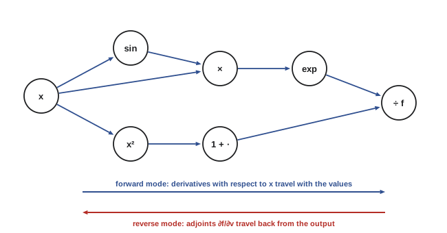
A program computing \(f\) can be written as a sequence of elementary operations, each with a known derivative: addition, multiplication, exp, sin, matrix multiplication, and so on. These form a directed acyclic graph from inputs to output. The chain rule says that the derivative of the output with respect to an input is the sum, over all paths through the graph, of the products of local derivatives along each path. Forward and reverse mode are two orders for computing that sum.

Forward mode

Forward mode attaches to every intermediate value \(v\) its derivative \(\dot{v} = \partial v/\partial x\) with respect to one chosen input, and propagates both together through each operation: for \(v = a \times b\), \(\dot{v} = \dot{a}b + a\dot{b}\). An elegant implementation uses dual numbers \(a + \dot{a}\varepsilon\) with \(\varepsilon^2 = 0\): arithmetic on dual numbers automatically applies the chain rule.

import math

class Dual:
    # a + b*eps with eps^2 = 0: carries a value and its derivative together
    def __init__(self, val, der=0.0):
        self.val, self.der = val, der
    def __add__(self, o):
        o = o if isinstance(o, Dual) else Dual(o)
        return Dual(self.val + o.val, self.der + o.der)
    __radd__ = __add__
    def __mul__(self, o):
        o = o if isinstance(o, Dual) else Dual(o)
        return Dual(self.val * o.val, self.der * o.val + self.val * o.der)
    __rmul__ = __mul__
    def __sub__(self, o):
        return self + (-1.0) * o
    def __truediv__(self, o):
        o = o if isinstance(o, Dual) else Dual(o)
        return Dual(self.val / o.val, (self.der * o.val - self.val * o.der) / o.val ** 2)

def exp(x):
    return Dual(math.exp(x.val), math.exp(x.val) * x.der)

def sin(x):
    return Dual(math.sin(x.val), math.cos(x.val) * x.der)

def f(x):
    return exp(sin(x) * x) / (1 + x * x)

x0 = 1.3
fx = f(Dual(x0, 1.0))                     # seed derivative dx/dx = 1
h = 1e-6
fd = (f(Dual(x0 + h)).val - f(Dual(x0 - h)).val) / (2 * h)
print(f"f(1.3) = {fx.val:.10f}")
print(f"forward-mode derivative  {fx.der:.10f}")
print(f"central difference       {fd:.10f}")

f(1.3) = 1.3009365751
forward-mode derivative  0.4485159825
central difference       0.4485159825

One forward pass gives the derivative of every output with respect to one input, so the full Jacobian of a function \(\mathbb{R}^n \to \mathbb{R}^m\) needs \(n\) passes. Forward mode is efficient when there are few inputs and many outputs, for example sensitivities of a simulation to a handful of parameters, or Jacobian-vector products \(Jv\) in a single pass.

Reverse mode and backpropagation

Reverse mode first runs the program forward, recording the graph and the intermediate values. It then sweeps backward from the output, computing for every node its adjoint \(\bar{v} = \partial f/\partial v\), the sensitivity of the output to that node. Each node passes its adjoint back to its inputs, multiplied by the local derivatives: for \(v = a \times b\), it adds \(\bar{v}b\) to \(\bar{a}\) and \(\bar{v}a\) to \(\bar{b}\). When the sweep reaches the inputs, their adjoints are the gradient.

One backward pass gives the derivative of one output with respect to all inputs, at a cost of a small multiple (typically two to four times) of the forward pass, regardless of the number of inputs. For training, where the output is a scalar loss and the inputs are millions or billions of parameters, this is exactly what is needed. Backpropagation in neural networks is reverse-mode AD applied to the network's computation.

import math
import random

class Value:
    # a scalar that records how it was computed, for reverse-mode differentiation
    def __init__(self, data, parents=(), local_grads=()):
        self.data, self.grad = data, 0.0
        self.parents, self.local_grads = parents, local_grads
    def __add__(self, o):
        o = o if isinstance(o, Value) else Value(o)
        return Value(self.data + o.data, (self, o), (1.0, 1.0))
    __radd__ = __add__
    def __mul__(self, o):
        o = o if isinstance(o, Value) else Value(o)
        return Value(self.data * o.data, (self, o), (o.data, self.data))
    __rmul__ = __mul__
    def tanh(self):
        t = math.tanh(self.data)
        return Value(t, (self,), (1 - t * t,))
    def backward(self):
        order, seen = [], set()
        def visit(v):
            if id(v) not in seen:
                seen.add(id(v))
                for p in v.parents:
                    visit(p)
                order.append(v)
        visit(self)
        self.grad = 1.0
        for v in reversed(order):                 # chain rule, from the output back
            for p, lg in zip(v.parents, v.local_grads):
                p.grad += lg * v.grad

random.seed(0)
# A tiny network: 3 inputs, 4 tanh hidden units, 1 output, squared error on one example
W1 = [[Value(random.uniform(-1, 1)) for _ in range(3)] for _ in range(4)]
W2 = [Value(random.uniform(-1, 1)) for _ in range(4)]
x, target = [0.5, -1.2, 2.0], 0.3

def loss():
    h = [sum((w * xi for w, xi in zip(row, x)), Value(0.0)).tanh() for row in W1]
    out = sum((w * hi for w, hi in zip(W2, h)), Value(0.0))
    d = out + (-target)
    return d * d

L = loss()
L.backward()
print(f"loss {L.data:.6f}")
# Check one weight against a finite difference
w = W1[2][1]
analytic = w.grad
eps = 1e-6
w.data += eps; up = loss().data
w.data -= 2 * eps; down = loss().data
w.data += eps
print(f"dL/dW1[2][1]: reverse mode {analytic:.8f}, finite difference {(up - down) / (2 * eps):.8f}")
n_params = 3 * 4 + 4
print(f"one backward pass gave all {n_params} gradients; finite differences would need {2 * n_params} loss evaluations")

loss 0.016675
dL/dW1[2][1]: reverse mode -0.04870060, finite difference -0.04870060
one backward pass gave all 16 gradients; finite differences would need 32 loss evaluations

Vector-Jacobian and Jacobian-vector products

In general, reverse mode computes vector-Jacobian products \(u^TJ\) and forward mode Jacobian-vector products \(Jv\), each for about the cost of one function evaluation. Combining them gives Hessian-vector products (forward over reverse), used by the second-order methods of Lesson 4. Libraries expose these as primitives (for example jvp and vjp in JAX), and higher derivatives by applying AD to AD.

The memory cost of reverse mode

Reverse mode must keep the intermediate values (activations) from the forward pass until the backward pass uses them. For a deep network, activation memory grows with depth, batch size and sequence length, and often exceeds the memory for the parameters themselves. Gradient checkpointing (rematerialization) stores only some activations, at checkpoints, and recomputes the rest during the backward pass from the nearest checkpoint.

import math
import numpy as np

# 1) Activation memory: store everything versus checkpoint every k layers
layers, act_mb = 96, 300.0          # layers and activation memory per layer for one microbatch, MB
for k in (1, 4, int(math.sqrt(layers)), 24):
    stored = layers if k == 1 else layers / k + k   # checkpoints kept plus one segment recomputed
    extra = 0 if k == 1 else 1       # roughly one extra forward pass when recomputing
    print(f"checkpoint every {k:2d} layers: about {stored * act_mb / 1000:5.1f} GB of activations, extra forward passes {extra}")

# 2) Gradients in 16-bit: small values underflow to zero unless the loss is scaled
rng = np.random.default_rng(0)
grads = np.abs(rng.normal(0, 1e-6, 100000)) * rng.choice([1e-2, 1, 1e2], 100000)
g16 = grads.astype(np.float16)
print(f"float16 smallest subnormal {np.finfo(np.float16).smallest_subnormal:.1e}; gradients flushed to zero: {np.mean(g16 == 0):.1%}")
scale = 2.0 ** 14
scaled = (grads * scale).astype(np.float16)
recovered = scaled.astype(np.float32) / scale
print(f"with loss scaling by 2^14: zeros {np.mean(scaled == 0):.1%}, median relative error {np.median(np.abs(recovered - grads) / grads):.1e}")
bf = (grads.astype(np.float32).view(np.uint32) & 0xFFFF0000).view(np.float32)   # bfloat16 by truncation
print(f"bfloat16 (8 exponent bits): zeros {np.mean(bf == 0):.1%}, median relative error {np.median(np.abs(bf - grads) / grads):.1e}")

checkpoint every  1 layers: about  28.8 GB of activations, extra forward passes 0
checkpoint every  4 layers: about   8.4 GB of activations, extra forward passes 1
checkpoint every  9 layers: about   5.9 GB of activations, extra forward passes 1
checkpoint every 24 layers: about   8.4 GB of activations, extra forward passes 1
float16 smallest subnormal 6.0e-08; gradients flushed to zero: 33.8%
with loss scaling by 2^14: zeros 0.0%, median relative error 1.8e-04
bfloat16 (8 exponent bits): zeros 0.0%, median relative error 2.7e-03

With checkpoints every \(\sqrt{L}\) layers, memory falls from proportional to \(L\) to about \(2\sqrt{L}\) layers' worth, at the cost of about one extra forward pass, roughly 30% more compute. Large-model training combines checkpointing with sharding of activations across devices (Lesson 12).

Precision

Gradients and activations are increasingly computed in 16-bit formats, which halve memory and run several times faster on modern accelerators:

• float16 has a 5-bit exponent, so its range is small: values below about \(6 \times 10^{-8}\) become zero. Many gradients are smaller than that. Loss scaling multiplies the loss by a large factor (such as \(2^{14}\)) before backpropagation, shifting gradients into the representable range, and divides them afterward; dynamic loss scaling adjusts the factor automatically, reducing it when overflows appear.
• bfloat16 keeps float32's 8-bit exponent with a shorter 7-bit mantissa, so it has the same range as float32 and needs no loss scaling, but less precision.
• Mixed precision keeps a float32 master copy of the weights and accumulates sums in float32, while computing matrix products in 16 bits, so that small updates are not lost when added to large weights.

Newer 8-bit formats (FP8) are used for parts of training on the latest hardware, with per-tensor or per-block scaling (Lesson 9 discusses precision and stability).

Checking gradients

Custom operations, hand-written backward functions, and numerical edge cases can produce wrong gradients that still let training proceed, slowly and badly. Gradient checking compares AD gradients with finite differences on a small example:

In float64 with central differences, relative errors around \(10^{-7}\) or smaller indicate a correct gradient; errors near \(10^{-2}\) or larger indicate a bug. Checks should be done in float64, on small inputs, at random points (not at zeros where many terms vanish), and away from kinks such as ReLU at 0, where finite differences are unreliable.

Differentiating through programs

Because AD works on programs, models can include loops, conditionals, solvers and simulations. Practical points:

• Control flow: AD differentiates the path actually taken; the derivative of a branch condition itself is zero.
• Non-differentiable points: frameworks pick a convention (the gradient of ReLU at 0 is usually 0), consistent with a subgradient (Lesson 2).
• Iterative solvers: differentiating through all iterations of an inner solver costs memory; implicit differentiation instead uses the optimality conditions of the solution, as in differentiable optimization layers and deep equilibrium models.
• Discrete operations such as sampling, rounding and argmax have zero or undefined gradients; estimators such as the reparameterization trick, straight-through estimators and score-function (REINFORCE) estimators provide useful surrogates.