Distributed optimization and a training project

Large models are trained on hundreds or thousands of accelerators at once, and some models are trained on data that cannot leave the devices or organizations that hold it. Both settings turn optimization into a problem of computation, memory and communication as much as mathematics. This final lesson explains data, tensor and pipeline parallelism, the memory accounting of large-model training and how sharding reduces it, the cost of communication and how optimizers cope with very large batches, asynchronous and federated optimization, and finally works through a training project that draws on the whole course, from choosing an optimizer to diagnosing problems.

Data parallelism

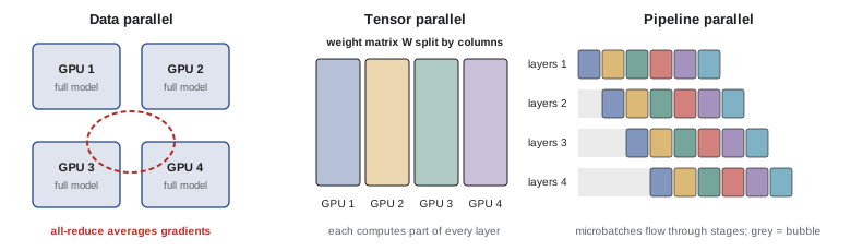
In synchronous data parallelism, each of \(N\) workers holds a copy of the model, processes a different minibatch, computes its gradient, and then all workers average their gradients with an all-reduce operation before each applies the same update. Mathematically this is ordinary minibatch SGD (Lesson 3) with an \(N\) times larger batch. Its limits are:

• Communication: every step exchanges a full set of gradients. A ring all-reduce sends about \(2(N-1)/N\) times the gradient size per worker, so communication time is roughly constant in \(N\) but proportional to model size and inversely proportional to network bandwidth.
• Large batches: beyond the critical batch size, more workers stop reducing the number of steps needed (Lesson 3), so adding workers adds cost without speeding training.
• Memory: each worker must hold the whole model, its gradients and its optimizer state.

Implementations overlap communication with computation, sending gradients of later layers while earlier layers are still being backpropagated, and use high-bandwidth interconnects (DCE-320) to keep accelerators busy.

Memory and sharding

Training with Adam in mixed precision (Lessons 5 and 6) stores, for each parameter, 16-bit weights and gradients and 32-bit master weights and two moment estimates: about 16 bytes per parameter, before activations. A 70-billion-parameter model needs over a terabyte for these alone, far beyond any single accelerator.

# Memory per GPU for training a 70-billion-parameter model with Adam in mixed precision
params = 70e9
bytes_weights16, bytes_grads16 = 2, 2
bytes_master32, bytes_m, bytes_v = 4, 4, 4
per_param = bytes_weights16 + bytes_grads16 + bytes_master32 + bytes_m + bytes_v
print(f"bytes per parameter: {per_param}; total {params * per_param / 1e9:,.0f} GB before activations")

gpus = 64
stages = {
    "plain data parallel": params * per_param,
    "ZeRO-1 (shard optimizer states)": params * (4 + (4 + 4 + 4) / gpus),
    "ZeRO-2 (+ shard gradients)": params * (2 + (2 + 4 + 4 + 4) / gpus),
    "ZeRO-3 / FSDP (+ shard weights)": params * per_param / gpus,
}
for name, b in stages.items():
    print(f"{name:34s}: {b / 1e9:8.1f} GB per GPU")

# Ring all-reduce time for the gradients of one step
grad_bytes = params * 2
bw = 400e9 / 8                        # 400 Gb/s per GPU, in bytes per second
t = 2 * (gpus - 1) / gpus * grad_bytes / bw
print(f"ring all-reduce of {grad_bytes / 1e9:.0f} GB of gradients across {gpus} GPUs: {t:.1f} s at 400 Gb/s")

bytes per parameter: 16; total 1,120 GB before activations
plain data parallel               :   1120.0 GB per GPU
ZeRO-1 (shard optimizer states)   :    293.1 GB per GPU
ZeRO-2 (+ shard gradients)        :    155.3 GB per GPU
ZeRO-3 / FSDP (+ shard weights)   :     17.5 GB per GPU
ring all-reduce of 140 GB of gradients across 64 GPUs: 5.5 s at 400 Gb/s

Sharding splits these states across workers instead of replicating them. ZeRO (zero redundancy optimizer) stage 1 shards the optimizer states, stage 2 also the gradients, and stage 3 (also known as fully sharded data parallel, FSDP) the weights themselves, gathering each layer's weights just before they are needed and discarding them afterwards. Stage 3 cuts per-device memory by the number of workers, at the cost of more communication.

Model parallelism

When even sharded data parallelism is not enough, the model itself is split:

• Tensor parallelism splits individual matrix multiplications across devices, for example dividing a layer's weight matrix by columns, so that each device computes part of every layer; it needs very fast communication, usually within a server.
• Pipeline parallelism assigns consecutive layers to different devices and streams microbatches through them, like an assembly line. Idle time at the start and end of each batch (the pipeline "bubble") is reduced by using many microbatches.
• Expert parallelism places the experts of mixture-of-experts layers on different devices, routing each token to the devices holding its chosen experts.
• Sequence or context parallelism splits long sequences across devices.

Large training runs combine several: tensor parallelism within servers, pipeline parallelism across a few servers, and sharded data parallelism across the rest, a configuration often called 3D or 4D parallelism. Choosing it is an optimization problem over memory, compute and the network topology (AI-480 covers it in depth).

Optimizers for very large batches

To use more workers effectively, practitioners push batch sizes up, which requires higher learning rates and careful stabilization:

• Learning rate scaling with warm-up: linear scaling for SGD up to the critical batch size, with gradual warm-up to avoid early instability (Lesson 3).
• Layer-wise adaptive rates: LARS (for SGD with momentum) and LAMB (for Adam) scale each layer's update by the ratio of its weight norm to its update norm, so no layer takes a disproportionately large step. They enabled training with batches of tens of thousands of examples.
• Gradient clipping and loss-spike handling (Lesson 5): at scale, rare instabilities can derail weeks of training, so runs monitor gradient norms and loss, skip or roll back bad steps, and restart from checkpoints.

Asynchronous and decentralized optimization

Synchronous training waits for the slowest worker at every step. Asynchronous methods let workers update a shared model (on parameter servers) without waiting, applying gradients computed on slightly stale weights. They tolerate stragglers but add noise from staleness; with modest delays and step sizes, they converge like SGD. Decentralized methods replace the central average with exchanges between neighbors in a communication graph (gossip averaging). Methods that communicate less often, such as local SGD (several local steps between averages) and DiLoCo-style training across loosely connected data centers, trade some optimization efficiency for far less communication.

Federated learning

In federated learning, data stays on clients (phones, hospitals, banks) and only model updates are shared. Federated averaging (FedAvg) sends the current model to a sample of clients, each runs several local SGD steps on its own data, and the server averages the returned models. Local steps reduce communication rounds, the scarce resource, but client data are usually not identically distributed, so local models drift toward their own optima.

import numpy as np

rng = np.random.default_rng(6)
d, clients = 10, 10
w_true = rng.normal(size=d)

def make_client(shift):
    X = rng.normal(size=(200, d)) + shift              # each client sees a different input distribution
    y = (X @ w_true + rng.normal(0, 0.5, 200) > 0).astype(float)
    return X, y

data = [make_client(rng.normal(0, 1.0, d)) for _ in range(clients)]
Xall = np.vstack([X for X, _ in data]); yall = np.concatenate([y for _, y in data])

def loss(w, X, y):
    z = X @ w
    return np.mean(np.logaddexp(0, z) - y * z)

def grad(w, X, y):
    return X.T @ (1 / (1 + np.exp(-X @ w)) - y) / len(y)

def fedavg(local_steps, rounds=30, lr=0.1):
    w = np.zeros(d)
    for _ in range(rounds):
        updates = []
        for X, y in data:
            wl = w.copy()
            for _ in range(local_steps):
                idx = rng.choice(len(y), 32)
                wl -= lr * grad(wl, X[idx], y[idx])
            updates.append(wl)
        w = np.mean(updates, axis=0)                   # the server averages client models
    return w

for steps in (1, 5, 25):
    w = fedavg(steps)
    print(f"{steps:2d} local steps per round, 30 rounds: global loss {loss(w, Xall, yall):.4f}, communication rounds 30")
w = np.zeros(d)
for _ in range(30 * 25):
    idx = rng.choice(len(yall), 32 * clients)
    w -= 0.1 * grad(w, Xall[idx], yall[idx])
print(f"centralized SGD, same total updates: global loss {loss(w, Xall, yall):.4f}")

 1 local steps per round, 30 rounds: global loss 0.3477, communication rounds 30
 5 local steps per round, 30 rounds: global loss 0.2016, communication rounds 30
25 local steps per round, 30 rounds: global loss 0.1204, communication rounds 30
centralized SGD, same total updates: global loss 0.1182

Here more local computation per round paid off, but with strongly heterogeneous clients, too many local steps make client models drift apart; methods such as FedProx and SCAFFOLD correct this drift. Federated learning is combined with secure aggregation, so the server sees only the sum of updates, and often with differential privacy (AI-220, Lesson 7), adding noise to updates to bound what can be learned about any one client.

Training project: putting the course together

Consider training a transformer language model of about 1 billion parameters on 100 billion tokens, on 64 accelerators. The steps show how the course's ideas combine:

• Objective and parameterization: next-token cross-entropy, a convex loss of the logits (Lesson 2); a parameterization such as μP so that hyperparameters tuned on small proxies transfer (Lesson 10).
• Optimizer: AdamW with \(\beta_1 = 0.9\), \(\beta_2 = 0.95\), weight decay 0.1 on matrices, gradient clipping at norm 1.0 (Lesson 5), in bfloat16 with float32 master weights (Lesson 6).
• Schedule: linear warm-up over about 2,000 steps, then cosine decay to 10% of the peak, or a constant rate with a final cooldown (Lesson 3).
• Batch size: chosen near the estimated critical batch size, perhaps 1 million tokens per step, giving about 100,000 steps (Lesson 3 and this lesson).
• Parallelism: sharded data parallelism (ZeRO-2 or FSDP) across 64 accelerators, with activation checkpointing if memory is tight (Lesson 6 and this lesson).
• Hyperparameters: peak learning rate and weight decay tuned with random search and early stopping on a 100-million-parameter proxy (Lesson 10).

Diagnosing training

During training, the curves tell what is happening:

• Loss spikes: often from learning rates that are too high for current sharpness (Lessons 1 and 9), or from bad data batches. Remedies: lower peak rate, longer warm-up, stronger clipping, skipping or rolling back.
• Divergence to NaN: overflow in low precision or exploding gradients. Check loss scaling (float16), clipping, and layer normalization placement.
• Plateau early in training: learning rate too low, poor initialization, or a bug; a learning-rate range test and a gradient check on a small model help (Lessons 6 and 10).
• Training loss falling, validation loss rising: overfitting, so more data, regularization or earlier stopping (Lesson 8).
• Slow throughput: communication bottlenecks or poor overlap; profile computation and communication separately.

Each diagnosis connects back to a principle: curvature and step size, noise and batch size, adaptivity and stability, regularization and generalization. Those principles, not any single recipe, are what let an engineer train a new model successfully.