Derivative-free, evolutionary and discrete optimization

Gradient-based methods dominate machine learning because gradients are cheap to compute by automatic differentiation (Lesson 6). Many important problems, however, offer no useful gradient: the objective may come from a simulator, a physical experiment or a compiled program; it may be noisy or discontinuous; or the variables may be discrete, such as a schedule, a route, a set of features or a neural architecture. This lesson surveys methods for such problems: direct search (Nelder-Mead, Powell), stochastic gradient estimates from function values (SPSA and zeroth-order methods), evolution strategies including CMA-ES, simulated annealing and local search for combinatorial problems, and an introduction to integer programming. It also shows where these methods appear in AI practice.

When gradients are not available

Situations without usable gradients include:

• Black-box objectives: the output of a simulation, a physical experiment, a compiled program, or an API whose internals are hidden.
• Non-differentiable or discontinuous objectives: accuracy rather than loss, step functions, quantized models.
• Noisy objectives where finite differences are swamped by noise.
• Discrete or combinatorial variables: routes, schedules, subsets, graph structures, architecture choices.
• Reinforcement learning environments, where the reward depends on the policy through an unknown environment (AI-330 develops policy gradients, which estimate gradients from samples).

Derivative-free methods use only function values. They typically need many more evaluations than gradient methods, and their cost grows with dimension, so they work best for problems with tens to a few thousand variables, or with structure that can be exploited.

Direct search: Nelder-Mead and Powell

The Nelder-Mead method keeps a simplex of \(d + 1\) points and repeatedly replaces the worst point by reflecting it through the centroid of the others, expanding if that helps, and contracting or shrinking if it does not. It adapts its shape to the function and is popular for small problems (a handful of parameters). It has no convergence guarantee in general and can stall, but it often works well in practice.

Powell's method performs a sequence of one-dimensional line searches along a set of directions, updating the directions to align with the valleys of the function. On smooth problems it can be very efficient.

import numpy as np
from scipy.optimize import minimize

rng = np.random.default_rng(3)
A = np.diag([1.0, 10.0, 100.0])

def f(x):
    return float(x @ A @ x)

def f_noisy(x):
    return f(x) + rng.normal(0, 0.01)

x0 = np.array([1.0, 1.0, 1.0])
for method in ("Nelder-Mead", "Powell"):
    r = minimize(f, x0, method=method, options={"xatol": 1e-6, "fatol": 1e-10, "maxfev": 5000} if method == "Nelder-Mead" else {"xtol": 1e-6, "ftol": 1e-10})
    print(f"{method:11s}: f = {r.fun:.1e} after {r.nfev} evaluations")

# (1+1) evolution strategy with the one-fifth success rule
x, sigma, fx, evals = x0.copy(), 0.5, f(x0), 1
while fx > 1e-10 and evals < 5000:
    y = x + sigma * rng.normal(size=3)
    fy = f(y); evals += 1
    if fy < fx:
        x, fx, sigma = y, fy, sigma * 1.5
    else:
        sigma *= 1.5 ** (-0.25)              # successes about 1/5 of the time keep sigma steady
print(f"(1+1)-ES    : f = {fx:.1e} after {evals} evaluations")

# SPSA: a gradient estimate from two evaluations, whatever the dimension, on a noisy objective
x = x0.copy()
for k in range(1, 3001):
    a, c = 0.008 / k ** 0.602, 0.1 / k ** 0.101
    delta = rng.choice([-1.0, 1.0], size=3)
    g = (f_noisy(x + c * delta) - f_noisy(x - c * delta)) / (2 * c) * delta
    x -= a * g
print(f"SPSA (noisy): f = {f(x):.1e} after {2 * 3000} evaluations")

Nelder-Mead: f = 1.7e-13 after 226 evaluations
Powell     : f = 2.6e-30 after 47 evaluations
(1+1)-ES    : f = 9.0e-11 after 936 evaluations
SPSA (noisy): f = 3.6e-03 after 6000 evaluations

Powell's method is fastest on this smooth problem; Nelder-Mead takes a few hundred evaluations; the evolution strategy takes about a thousand but needs no assumptions about smoothness; SPSA makes steady progress despite noise that would defeat finite differences.

Gradient estimates from function values

A gradient can be estimated from function values alone. Finite differences need \(d + 1\) or \(2d\) evaluations per estimate, which is expensive in high dimensions and fragile with noise. Randomized estimates cost far less per step:

• SPSA (simultaneous perturbation stochastic approximation) perturbs all coordinates at once with a random \(\pm 1\) vector \(\Delta\) and uses two evaluations: \(\hat{g} = \frac{f(x + c\Delta) - f(x - c\Delta)}{2c}\Delta\). The estimate is noisy but unbiased in expectation (to first order), whatever the dimension.
• Gaussian smoothing estimates the gradient of a smoothed version of \(f\) from random Gaussian directions, the basis of zeroth-order optimization and of evolution strategies used for policy search.

With decreasing step sizes and perturbation sizes, these methods converge like stochastic gradient descent, though more slowly by a factor that grows with dimension. They are used for tuning controllers, calibrating simulators, adversarial attacks on black-box models, and fine-tuning when memory does not allow backpropagation.

Evolution strategies and CMA-ES

Evolution strategies (ES) maintain a search distribution, usually Gaussian, sample candidate points from it, evaluate them, and move the distribution toward the better ones. The simplest, the (1+1)-ES, mutates one parent and keeps the child if it is better, adapting the step size by the one-fifth success rule: increase it if more than a fifth of mutations succeed, decrease it otherwise.

The covariance matrix adaptation evolution strategy (CMA-ES) is the state of the art for continuous black-box problems of moderate dimension (up to a few hundred variables). Each generation it samples \(\lambda\) points from \(\mathcal{N}(m, \sigma^2 C)\), ranks them, moves the mean toward the best, and updates the covariance \(C\) so that the distribution stretches along directions of past success. Over time \(C\) learns an approximation of the inverse Hessian, so CMA-ES handles ill-conditioned and rotated problems that defeat coordinate-wise methods. It is invariant to monotone transformations of the objective, since it uses only rankings, and robust to moderate noise.

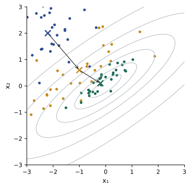
Large-scale variants of evolution strategies have been used to train neural network policies for reinforcement learning on thousands of processors, because each worker needs only to report a scalar return, making communication cheap.

Combinatorial optimization: local search and simulated annealing

Discrete problems, such as routing, scheduling, assignment, feature selection and graph partitioning, often have astronomically many candidate solutions: a traveling salesperson tour of 25 cities can be chosen in \(24!/2 \approx 3 \times 10^{23}\) ways. Exact methods exist for many such problems (below), but heuristics give good solutions quickly:

• Local search moves between neighboring solutions, such as tours that differ by reversing one segment (a 2-opt move), accepting improvements until none remain. It finds a local optimum, which depends on the start.
• Simulated annealing also accepts some worsening moves, with probability \(e^{-\Delta/T}\) for a worsening \(\Delta\) at temperature \(T\), and slowly lowers \(T\). Early on it explores widely; later it behaves like local search. With slow enough cooling it can escape local optima.
• Tabu search, genetic algorithms, and large-neighborhood search are other widely used metaheuristics.

import numpy as np

# Simulated annealing on a 25-city travelling salesperson problem
rng = np.random.default_rng(11)
pts = rng.random((25, 2))
D = np.sqrt(((pts[:, None, :] - pts[None, :, :]) ** 2).sum(-1))

def length(tour):
    return D[tour, np.roll(tour, -1)].sum()

# Greedy nearest-neighbour tour as a baseline
tour = [0]
while len(tour) < 25:
    last = tour[-1]
    tour.append(min((j for j in range(25) if j not in tour), key=lambda j: D[last, j]))
tour = np.array(tour)
print(f"nearest-neighbour tour length {length(tour):.3f}")

# 2-opt moves: reverse a segment; accept worse tours with probability exp(-delta / T)
best, cur, cur_len = tour.copy(), tour.copy(), length(tour)
best_len, T = cur_len, 0.5
for step in range(60000):
    i, j = sorted(rng.choice(25, 2, replace=False))
    cand = cur.copy(); cand[i:j + 1] = cand[i:j + 1][::-1]
    delta = length(cand) - cur_len
    if delta < 0 or rng.random() < np.exp(-delta / T):
        cur, cur_len = cand, cur_len + delta
        if cur_len < best_len:
            best, best_len = cur.copy(), cur_len
    T *= 0.9999
print(f"simulated annealing best tour {best_len:.3f} (final temperature {T:.4f})")

# Greedy 2-opt (no uphill moves) from the same start, for comparison
cur, cur_len = tour.copy(), length(tour)
improved = True
while improved:
    improved = False
    for i in range(1, 24):
        for j in range(i + 1, 25):
            cand = cur.copy(); cand[i:j + 1] = cand[i:j + 1][::-1]
            if length(cand) < cur_len - 1e-12:
                cur, cur_len, improved = cand, length(cand), True
print(f"greedy 2-opt local optimum {cur_len:.3f}")

nearest-neighbor tour length 4.880
simulated annealing best tour 4.184 (final temperature 0.0012)
greedy 2-opt local optimum 4.232

Simulated annealing improves on the greedy tour by about 14%, and slightly beats pure local search from the same start, which stopped at a local optimum. On larger problems, the gap between good heuristics and naive ones grows, and well-tuned specialized heuristics (such as Lin-Kernighan for the traveling salesperson problem) find tours within a fraction of a percent of optimal.

Integer and mixed-integer programming

When a discrete problem can be written with linear objectives and constraints over integer and continuous variables, mixed-integer linear programming (MILP) solvers can find provably optimal solutions, or solutions with a guaranteed bound on how far from optimal they are. They combine the linear programming relaxation (Lesson 7), which gives a bound, with branch and bound, which splits the problem on fractional variables, and cutting planes, which tighten the relaxation. Modern solvers (commercial ones such as Gurobi and CPLEX, and open-source ones such as HiGHS and SCIP) solve problems with millions of variables in practice, despite worst-case exponential complexity.

In machine learning, integer programming appears in scheduling jobs on clusters, placing model shards on devices, selecting features with exact cardinality constraints, verifying neural networks, and in operations research problems that consume model predictions.

Choosing a method

• Smooth, cheap, differentiable: use gradients.
• A few continuous parameters, expensive and smooth: Bayesian optimization (Lesson 10), Powell or Nelder-Mead.
• Tens to hundreds of continuous parameters, noisy or rugged: CMA-ES or SPSA.
• Combinatorial with good modeling structure: MILP or constraint programming.
• Combinatorial and huge or poorly structured: local search, simulated annealing or other metaheuristics, often seeded with a greedy solution.

Hybrids are common: gradient methods for continuous parts and discrete search for structure, as in neural architecture search, or learned heuristics inside solvers.